截断和折叠分布
本教程将介绍如何在 NumPyro 中处理截断和折叠分布。假定您已熟悉 NumPyro 的基础知识。为了充分利用本教程,您需要具备一些概率论背景。
目录
设置
要运行此 notebook,我们需要导入以下内容
[ ]:
!pip install -q git+https://github.com/pyro-ppl/numpyro.git
[2]:
import matplotlib.pyplot as plt
import numpy as np
from scipy.stats import poisson as sp_poisson

import jax
from jax import lax, random
import jax.numpy as jnp
from jax.scipy.special import ndtri
from jax.scipy.stats import norm, poisson

import numpyro
import numpyro.distributions as dist
from numpyro.distributions import (
    Distribution,
    FoldedDistribution,
    SoftLaplace,
    StudentT,
    TruncatedDistribution,
    TruncatedNormal,
    constraints,
)
from numpyro.distributions.util import promote_shapes
from numpyro.infer import MCMC, NUTS, DiscreteHMCGibbs, Predictive

numpyro.enable_x64()
RNG = random.PRNGKey(0)
PRIOR_RNG, MCMC_RNG, PRED_RNG = random.split(RNG, 3)
MCMC_KWARGS = dict(
    num_warmup=2000,
    num_samples=2000,
    num_chains=4,
    chain_method="sequential",
)
1. 什么是截断分布?
概率分布的支撑集是域中概率非零的值集合。例如,正态分布的支撑集是整个实数线(即使密度随着远离均值而变得非常小,但从技术上讲,它永远不会完全为零)。均匀分布的支撑集,如在默认参数下编码的 jax.random.uniform 中所示,是区间 \(\left[0, 1)\right.\),因为该区间之外的任何值概率都为零。泊松分布的支撑集是非负整数集合,等等。
截断分布会使其支撑集变小,从而使任何超出我们期望域的值概率为零。在实践中,这对于模拟数据收集过程中引入某些偏差的情况很有用。例如,一些物理探测器仅在信号高于某个最小阈值时触发,或者有时如果信号超过某个值,探测器就会失效。结果,观测值被限制在有限的数值范围内,即使真实信号没有相同的限制。例如,参见 David Mackay 的《信息论与学习算法》第 3.1 节。朴素地看,如果 \(S\) 是原始密度 \(p_Y(y)\) 的支撑集,那么通过截断到新的支撑集 \(T\subset S\),我们实际上定义了一个新的随机变量 \(Z\),其密度为
写 \(\propto\)(正比于)符号而不是严格等号的原因在于,按上述方式定义,所得函数积分不为 \(1\),因此它不能严格地被视为概率密度。为了使其成为概率密度,我们需要将截断的质量重新分配到分布的剩余部分。为此,我们只需用同一个常数重新加权每个点
其中 \(M = \int_T p_Y(y)\mathrm{d}y\)。
在实践中,截断通常是单侧的。这意味着,例如,如果截断前的支撑集是区间 \((a, b)\),那么截断后的支撑集形式为 \((a, c)\) 或 \((c, b)\),其中 \(a < c < b\)。下图展示了正态分布 \(N(1, 1)\) 在零处的左侧截断。

原始分布(左侧)在垂直虚线处被截断。截断的质量(橙色区域)在新的支撑集(右侧图像)中被重新分配,以便即使截断后曲线下的总面积仍等于 1。这种重新加权的方法确保了任何两点之间的密度比 \(p(a)/p(b)\) 在重新加权前后保持不变(当然,只要这些点在新支撑集内)。
注意:截断数据不同于审查数据。审查也会隐藏超出某个期望支撑集的值,但与截断数据不同的是,我们知道何时发生了审查。典型的例子是家用秤,它不会报告超过 300 磅的值。本教程不涵盖审查数据。
2. 什么是折叠分布?
折叠是通过取随机变量的绝对值来实现的,\(Z = \lvert Y \rvert\)。这显然改变了原始分布的支撑集,因为负值现在概率为零
下图展示了折叠正态分布 \(N(1, 1)\)。

如您所见,所得分布与截断情况不同。特别是,点之间的密度比 \(p(a)/p(b)\) 在折叠后通常不同。有关折叠相关的一些示例,请参见参考文献 3 和 4
如果原始分布关于零对称,那么在零处折叠和截断具有相同的效果。
3. 从截断和折叠分布中采样
截断分布
通常,我们已经有了预截断分布的采样器(例如 np.random.normal)。因此,一种看似简单的方法来从截断分布生成样本是先从原始分布采样,然后丢弃超出期望支撑集的样本。例如,如果我们要从截断到支撑集 \((-\infty, 1)\) 的正态分布中采样,我们只需这样做
upper = 1
samples = np.random.normal(size=1000)
truncated_samples = samples[samples < upper]
这称为拒绝采样,但效率不高。如果我们截断的区域具有足够高的概率质量,那么我们将丢弃大量样本,可能需要一段时间才能为截断分布积累足够的样本。例如,上述代码片段尽管我们最初抽取了 1000 个样本,但只会产生大约 840 个截断样本。对于其他参数组合,这种情况很容易变得更糟。一种更有效的方法是使用称为逆变换采样的方法。在这种方法中,我们首先从 (0, 1) 范围内的均匀分布中采样,然后使用我们截断分布的逆累积分布函数来变换这些样本。这种方法确保在此过程中没有样本被浪费,尽管它确实有一个小小的复杂性,即我们需要计算我们截断分布的逆 CDF (ICDF)。这乍一听可能太复杂,但经过一些代数运算,我们通常可以根据未截断的 ICDF 计算截断的 ICDF。许多分布的未截断 ICDF 已经可用。
折叠分布
这种情况要简单得多。由于我们已经有了预折叠分布的采样器,我们所需要做的就是取这些样本的绝对值
samples = np.random.normal(size=1000)
folded_samples = np.abs(samples)
4. 现成的截断和折叠分布
4. 可直接使用的截断和折叠分布
本教程后面的部分将向您展示如何构建您自己的截断和折叠分布,但您不必重复造轮子。NumPyro 已经实现了许多截断分布。例如,假设您想要一个右截断的正态分布。为此,我们使用 TruncatedNormal 分布。此分布的参数是 loc 和 scale,对应于未截断正态分布的 loc 和 scale,以及对应于截断点的 low 和/或 high。重要的是,low 和 high 仅为关键字参数,只有 loc 和 scale 可以作为位置参数使用。您可以在模型中这样使用此类
[3]:
def truncated_normal_model(num_observations, high, x=None):
    loc = numpyro.sample("loc", dist.Normal())
    scale = numpyro.sample("scale", dist.LogNormal())
    with numpyro.plate("observations", num_observations):
        numpyro.sample("x", TruncatedNormal(loc, scale, high=high), obs=x)
现在我们来检查一下,我们是否可以在典型的 MCMC 工作流程中使用此模型。
先验模拟
[4]:
high = 1.2
num_observations = 250
num_prior_samples = 100

prior = Predictive(truncated_normal_model, num_samples=num_prior_samples)
prior_samples = prior(PRIOR_RNG, num_observations, high)
推断
为了测试我们的模型,我们针对一些合成数据运行 MCMC。合成数据可以是先验模拟中的任意样本。
[5]:
# -- select an arbitrary prior sample as true data
true_idx = 0
true_loc = prior_samples["loc"][true_idx]
true_scale = prior_samples["scale"][true_idx]
true_x = prior_samples["x"][true_idx]
[6]:
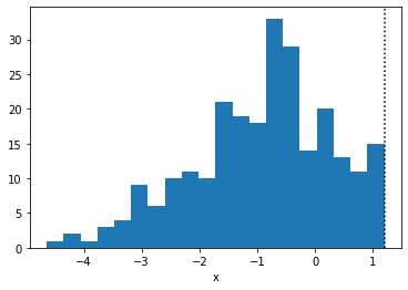
plt.hist(true_x.copy(), bins=20)
plt.axvline(high, linestyle=":", color="k")
plt.xlabel("x")
plt.show()
[7]:
# --- Run MCMC and check estimates and diagnostics
mcmc = MCMC(NUTS(truncated_normal_model), **MCMC_KWARGS)
mcmc.run(MCMC_RNG, num_observations, high, true_x)
mcmc.print_summary()

# --- Compare to ground truth
print(f"True loc  : {true_loc:3.2}")
print(f"True scale: {true_scale:3.2}")
sample: 100%|█████████████████████████████████████████████████████████████████████████████████████████████████████████████████████████| 4000/4000 [00:02<00:00, 1909.24it/s, 1 steps of size 5.65e-01. acc. prob=0.93]
sample: 100%|████████████████████████████████████████████████████████████████████████████████████████████████████████████████████████| 4000/4000 [00:00<00:00, 10214.14it/s, 3 steps of size 5.16e-01. acc. prob=0.95]
sample: 100%|████████████████████████████████████████████████████████████████████████████████████████████████████████████████████████| 4000/4000 [00:00<00:00, 15102.95it/s, 1 steps of size 6.42e-01. acc. prob=0.90]
sample: 100%|████████████████████████████████████████████████████████████████████████████████████████████████████████████████████████| 4000/4000 [00:00<00:00, 16522.03it/s, 3 steps of size 6.39e-01. acc. prob=0.90]
                mean       std    median      5.0%     95.0%     n_eff     r_hat
       loc     -0.58      0.15     -0.59     -0.82     -0.35   2883.69      1.00
     scale      1.49      0.11      1.48      1.32      1.66   3037.78      1.00

Number of divergences: 0
True loc  : -0.56
True scale: 1.4
移除截断
一旦我们推断出模型的参数,一项常见的任务是理解数据在没有截断的情况下会是什么样子。在此示例中,只需简单地将 high 的值“推”到无穷大即可轻松完成此操作。
[8]:
pred = Predictive(truncated_normal_model, posterior_samples=mcmc.get_samples())
pred_samples = pred(PRED_RNG, num_observations, high=float("inf"))
最后,绘制这些样本并将其与原始观测数据进行比较。
[9]:
# thin the samples to not saturate matplotlib
samples_thinned = pred_samples["x"].ravel()[::1000]
[10]:
f, axes = plt.subplots(1, 2, figsize=(15, 5), sharex=True)

axes[0].hist(
    samples_thinned.copy(), label="Untruncated posterior", bins=20, density=True
)
axes[0].set_title("Untruncated posterior")

vals, bins, _ = axes[1].hist(
    samples_thinned[samples_thinned < high].copy(),
    label="Tail of untruncated posterior",
    bins=10,
    density=True,
)
axes[1].hist(
    true_x.copy(), bins=bins, label="Observed, truncated data", density=True, alpha=0.5
)
axes[1].set_title("Comparison to observed data")

for ax in axes:
    ax.axvline(high, linestyle=":", color="k", label="Truncation point")
    ax.legend()

plt.show()
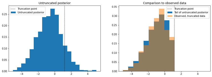
左侧的图显示了移除截断后从后验分布中模拟的数据,因此我们可以看到如果数据没有截断会是什么样子。为了进行合理性检查,我们丢弃高于截断点的模拟样本,绘制这些样本的直方图,并将其与真实数据(右侧图)的直方图进行比较。
TruncatedDistribution 类
NumPyro 中 TruncatedNormal 的源代码使用了一个名为 TruncatedDistribution 的类,该类抽象了我们将在下一节讨论的 sample 和 log_prob 逻辑。不过,目前此逻辑仅适用于具有实数支撑集的连续对称分布。
我们可以使用此类快速构建其他截断分布。例如,如果我们需要一个截断的 SoftLaplace 分布,我们可以使用以下模式
[11]:
def TruncatedSoftLaplace(
    loc=0.0, scale=1.0, *, low=None, high=None, validate_args=None
):
    return TruncatedDistribution(
        base_dist=SoftLaplace(loc, scale),
        low=low,
        high=high,
        validate_args=validate_args,
    )
[12]:
def truncated_soft_laplace_model(num_observations, high, x=None):
    loc = numpyro.sample("loc", dist.Normal())
    scale = numpyro.sample("scale", dist.LogNormal())
    with numpyro.plate("obs", num_observations):
        numpyro.sample("x", TruncatedSoftLaplace(loc, scale, high=high), obs=x)
并且,如前所述,我们检查我们可以在典型工作流程的步骤中使用此模型
[13]:
high = 2.3
num_observations = 200
num_prior_samples = 100

prior = Predictive(truncated_soft_laplace_model, num_samples=num_prior_samples)
prior_samples = prior(PRIOR_RNG, num_observations, high)

true_idx = 0
true_x = prior_samples["x"][true_idx]
true_loc = prior_samples["loc"][true_idx]
true_scale = prior_samples["scale"][true_idx]

mcmc = MCMC(
    NUTS(truncated_soft_laplace_model),
    **MCMC_KWARGS,
)

mcmc.run(
    MCMC_RNG,
    num_observations,
    high,
    true_x,
)

mcmc.print_summary()

print(f"True loc  : {true_loc:3.2}")
print(f"True scale: {true_scale:3.2}")
sample: 100%|█████████████████████████████████████████████████████████████████████████████████████████████████████████████████████████| 4000/4000 [00:02<00:00, 1745.70it/s, 1 steps of size 6.78e-01. acc. prob=0.93]
sample: 100%|█████████████████████████████████████████████████████████████████████████████████████████████████████████████████████████| 4000/4000 [00:00<00:00, 9294.56it/s, 1 steps of size 7.02e-01. acc. prob=0.93]
sample: 100%|████████████████████████████████████████████████████████████████████████████████████████████████████████████████████████| 4000/4000 [00:00<00:00, 10412.30it/s, 1 steps of size 7.20e-01. acc. prob=0.92]
sample: 100%|████████████████████████████████████████████████████████████████████████████████████████████████████████████████████████| 4000/4000 [00:00<00:00, 10583.85it/s, 3 steps of size 7.01e-01. acc. prob=0.93]
                mean       std    median      5.0%     95.0%     n_eff     r_hat
       loc     -0.37      0.17     -0.38     -0.65     -0.10   4034.96      1.00
     scale      1.46      0.12      1.45      1.27      1.65   3618.77      1.00

Number of divergences: 0
True loc  : -0.56
True scale: 1.4
重要
TruncatedDistribution 类的 sample 方法依赖于逆变换采样。这隐含要求基础分布已提供 icdf 方法。如果不是这样,我们将无法在我们的分布的任何实例上调用 sample 方法,也无法将其与 Predictive 类一起使用。然而,log_prob 方法仅依赖于 cdf 方法(该方法比 icdf 更常可用)。如果 log_prob 方法可用,那么我们可以在模型中将我们的分布用作先验/似然。
The FoldedDistribution class
与截断分布类似,NumPyro 提供了 FoldedDistribution 类,帮助您快速构建折叠分布。常见的折叠分布示例有所谓的“半正态”、“半学生”或“半柯西”分布。顾名思义,这些分布只保留分布的(正的)一半。这些“半”分布名称中隐含着它们在折叠前以零为中心。但是,当然,即使分布不以零为中心,您也可以对其进行折叠。例如,您可以像这样定义折叠学生 t 分布。
[14]:
def FoldedStudentT(df, loc=0.0, scale=1.0):
    return FoldedDistribution(StudentT(df, loc=loc, scale=scale))
[15]:
def folded_student_model(num_observations, x=None):
    df = numpyro.sample("df", dist.Gamma(6, 2))
    loc = numpyro.sample("loc", dist.Normal())
    scale = numpyro.sample("scale", dist.LogNormal())
    with numpyro.plate("obs", num_observations):
        numpyro.sample("x", FoldedStudentT(df, loc, scale), obs=x)
我们检查我们可以在典型工作流程中使用我们的分布
[16]:
# --- prior sampling
num_observations = 500
num_prior_samples = 100
prior = Predictive(folded_student_model, num_samples=num_prior_samples)
prior_samples = prior(PRIOR_RNG, num_observations)


# --- choose any prior sample as the ground truth
true_idx = 0
true_df = prior_samples["df"][true_idx]
true_loc = prior_samples["loc"][true_idx]
true_scale = prior_samples["scale"][true_idx]
true_x = prior_samples["x"][true_idx]

# --- do inference with MCMC
mcmc = MCMC(
    NUTS(folded_student_model),
    **MCMC_KWARGS,
)
mcmc.run(MCMC_RNG, num_observations, true_x)

# --- Check diagostics
mcmc.print_summary()

# --- Compare to ground truth:
print(f"True df   : {true_df:3.2f}")
print(f"True loc  : {true_loc:3.2f}")
print(f"True scale: {true_scale:3.2f}")
sample: 100%|█████████████████████████████████████████████████████████████████████████████████████████████████████████████████████████| 4000/4000 [00:02<00:00, 1343.54it/s, 7 steps of size 3.51e-01. acc. prob=0.75]
sample: 100%|█████████████████████████████████████████████████████████████████████████████████████████████████████████████████████████| 4000/4000 [00:01<00:00, 3644.99it/s, 7 steps of size 3.56e-01. acc. prob=0.73]
sample: 100%|█████████████████████████████████████████████████████████████████████████████████████████████████████████████████████████| 4000/4000 [00:01<00:00, 3137.13it/s, 7 steps of size 2.62e-01. acc. prob=0.91]
sample: 100%|█████████████████████████████████████████████████████████████████████████████████████████████████████████████████████████| 4000/4000 [00:01<00:00, 3028.93it/s, 7 steps of size 1.85e-01. acc. prob=0.96]
                mean       std    median      5.0%     95.0%     n_eff     r_hat
        df      3.12      0.52      3.07      2.30      3.97   2057.60      1.00
       loc     -0.02      0.88     -0.03     -1.28      1.34    925.84      1.01
     scale      2.23      0.21      2.25      1.89      2.57   1677.38      1.00

Number of divergences: 33
True df   : 3.01
True loc  : 0.37
True scale: 2.41
5. 构建您自己的截断分布
如果 TruncatedDistribution 和 FoldedDistribution 类不足以解决您的问题,您可能需要考虑从头开始编写自己的截断分布。这可能是一个繁琐的过程,因此本节将提供一些指导和示例来帮助您完成此任务。
5.1 NumPyro 分布回顾
NumPyro 分布应继承自 Distribution 并实现一些基本要素
类属性
类属性有多种用途。在这里,我们将主要关注两个
arg_constraints:对分布的参数施加一些要求。如果传递的参数不满足约束,则在实例化时引发错误。support:在某些推断算法(如 MCMC 和带 auto-guides 的 SVI)中使用,我们需要在无约束空间中执行算法。了解支撑集后,我们可以在底层自动进行参数重整化。
我们将逐步解释其他类属性。
__init__ 方法
这里是我们定义分布参数的地方。我们还使用 jax 和 lax 将参数提升到对广播有效的形状。父类的 __init__ 方法也是必需的,因为参数的验证是在那里完成的。
log_prob 方法
实现 log_prob 方法确保我们可以进行推断。顾名思义,此方法返回在参数处评估的密度的对数。
sample 方法
此方法用于从我们的分布中抽取独立样本。它对于进行先验和后验预测检查特别有用。特别注意,如果您只需要在模型中将分布用作先验,则不需要此方法 - log_prob 方法就足够了。
我们任何实现的占位符代码都可以写成
class MyDistribution(Distribution):
    # class attributes
    arg_constraints = {}
    support = None
    def __init__(self):
        pass

    def log_prob(self, value):
        pass

    def sample(self, key, sample_shape=()):
        pass
5.2 示例:右截断正态分布
我们将修改正态分布,使其新支撑集的形式为 (-inf, high),其中 high 是一个实数。这可以使用 TruncatedNormal 分布来完成,但为了演示起见,我们不依赖它。我们将我们的分布命名为 RightTruncatedNormal。让我们编写骨架代码,然后继续填补空白。
class RightTruncatedNormal(Distribution):
    # <class attributes>
    def __init__(self):
        pass

    def log_prob(self, value):
        pass

    def sample(self, key, sample_shape=()):
        pass
类属性
记住,在 NumPyro 中,未截断正态分布由两个参数指定,loc 和 scale,分别对应于均值和标准差。查看 Normal 分布的源代码,我们看到以下几行
arg_constraints = {"loc": constraints.real, "scale": constraints.positive}
support = constraints.real
reparametrized_params = ["loc", "scale"]
reparametrized_params 属性在构建梯度估计器时被变分推断算法使用。许多具有连续支撑集的常见分布(例如正态分布)的参数是可重参数化的,而离散分布的参数则不是。请注意,reparametrized_params 对于 HMC 等 MCMC 算法无关紧要。更多详情请参见SVI 第三部分。
我们必须通过包含 "high" 参数来适应我们的情况,但我们需要处理两个问题
constraints.real有点过于严格。我们希望jnp.inf对于high是一个有效值(相当于没有截断),但目前无穷大不是有效的实数。我们通过定义自己的约束来处理这种情况。constraints.real的源代码很容易模仿
class _RightExtendedReal(constraints.Constraint):
    """
    Any number in the interval (-inf, inf].
    """
    def __call__(self, x):
        return (x == x) & (x != float("-inf"))

    def feasible_like(self, prototype):
        return jnp.zeros_like(prototype)

right_extended_real = _RightExtendedReal()
support不能再是一个类属性,因为它将依赖于high的值。因此,我们将其实现为一个依赖属性。
我们的分布看起来如下
class RightTruncatedNormal(Distribution):
    arg_constraints = {
        "loc": constraints.real,
        "scale": constraints.positive,
        "high": right_extended_real,
    }
    reparametrized_params = ["loc", "scale", "high"]

    # ...

    @constraints.dependent_property
    def support(self):
        return constraints.lower_than(self.high)
__init__ 方法
我们再次借鉴了正态分布的源代码。关键在于使用 lax 和 jax 来检查传递参数的形状,并确保这些形状对于广播是一致的。我们在我们的用例中遵循相同的模式——我们所需要做的就是包含 high 参数。
在 Normal 的源代码实现中,参数 loc 和 scale 都设置了默认值,这样在未指定参数时可以得到标准正态分布。同样地,我们选择 float("inf") 作为 high 的默认值,这等同于没有截断。
# ...
    def __init__(self, loc=0.0, scale=1.0, high=float("inf"), validate_args=None):
        batch_shape = lax.broadcast_shapes(
            jnp.shape(loc),
            jnp.shape(scale),
            jnp.shape(high),
        )
        self.loc, self.scale, self.high = promote_shapes(loc, scale, high)
        super().__init__(batch_shape, validate_args=validate_args)
# ...
log_prob 方法
对于截断分布,对数密度由下式给出
其中,再次强调,\(p_Z\) 是截断分布的密度,\(p_Y\) 是截断前的密度,\(M = \int_T p_Y(y)\mathrm{d}y\)。对于将正态分布截断到区间 (-inf, high) 的特定情况,常数 \(M\) 等于在截断点评估的累积密度。我们可以轻松实现此对数密度方法,因为 jax.scipy.stats 已经有一个我们可以使用的 norm 模块。
# ...
    def log_prob(self, value):
        log_m = norm.logcdf(self.high, self.loc, self.scale)
        log_p = norm.logpdf(value, self.loc, self.scale)
        return jnp.where(value < self.high, log_p - log_m, -jnp.inf)
# ...
sample 方法
为了使用逆变换采样实现 sample 方法,我们还需要实现逆累积分布函数。为此,我们可以使用 jax.scipy.special 中的 ndtri 函数。此函数返回标准正态分布的逆 CDF。我们可以进行一些代数运算来获得截断的非标准正态分布的逆 CDF。首先回想一下,如果 \(X\sim Normal(0, 1)\) 且 \(Y = \mu + \sigma X\),则 \(Y\sim Normal(\mu, \sigma)\)。那么,如果 \(Z\) 是截断的 \(Y\),其累积密度由下式给出
因此其逆函数为
上述数学公式翻译成代码如下
# ...
    def sample(self, key, sample_shape=()):
        shape = sample_shape + self.batch_shape
        minval = jnp.finfo(jnp.result_type(float)).tiny
        u = random.uniform(key, shape, minval=minval)
        return self.icdf(u)


    def icdf(self, u):
        m = norm.cdf(self.high, self.loc, self.scale)
        return self.loc + self.scale * ndtri(m * u)
一切就绪后,最终实现如下所示。
[17]:
class _RightExtendedReal(constraints.Constraint):
    """
    Any number in the interval (-inf, inf].
    """

    def __call__(self, x):
        return (x == x) & (x != float("-inf"))

    def feasible_like(self, prototype):
        return jnp.zeros_like(prototype)


right_extended_real = _RightExtendedReal()


class RightTruncatedNormal(Distribution):
    """
    A truncated Normal distribution.
    :param numpy.ndarray loc: location parameter of the untruncated normal
    :param numpy.ndarray scale: scale parameter of the untruncated normal
    :param numpy.ndarray high: point at which the truncation happens
    """

    arg_constraints = {
        "loc": constraints.real,
        "scale": constraints.positive,
        "high": right_extended_real,
    }
    reparametrized_params = ["loc", "scale", "high"]

    def __init__(self, loc=0.0, scale=1.0, high=float("inf"), validate_args=True):
        batch_shape = lax.broadcast_shapes(
            jnp.shape(loc),
            jnp.shape(scale),
            jnp.shape(high),
        )
        self.loc, self.scale, self.high = promote_shapes(loc, scale, high)
        super().__init__(batch_shape, validate_args=validate_args)

    def log_prob(self, value):
        log_m = norm.logcdf(self.high, self.loc, self.scale)
        log_p = norm.logpdf(value, self.loc, self.scale)
        return jnp.where(value < self.high, log_p - log_m, -jnp.inf)

    def sample(self, key, sample_shape=()):
        shape = sample_shape + self.batch_shape
        minval = jnp.finfo(jnp.result_type(float)).tiny
        u = random.uniform(key, shape, minval=minval)
        return self.icdf(u)

    def icdf(self, u):
        m = norm.cdf(self.high, self.loc, self.scale)
        return self.loc + self.scale * ndtri(m * u)

    @constraints.dependent_property
    def support(self):
        return constraints.less_than(self.high)
试试看!
[18]:
def truncated_normal_model(num_observations, x=None):
    loc = numpyro.sample("loc", dist.Normal())
    scale = numpyro.sample("scale", dist.LogNormal())
    high = numpyro.sample("high", dist.Normal())
    with numpyro.plate("observations", num_observations):
        numpyro.sample("x", RightTruncatedNormal(loc, scale, high), obs=x)
[19]:
num_observations = 1000
num_prior_samples = 100
prior = Predictive(truncated_normal_model, num_samples=num_prior_samples)
prior_samples = prior(PRIOR_RNG, num_observations)
如前所述,我们针对一些合成数据运行 mcmc。我们从先验中选择任意随机样本作为真实值
[20]:
true_idx = 0
true_loc = prior_samples["loc"][true_idx]
true_scale = prior_samples["scale"][true_idx]
true_high = prior_samples["high"][true_idx]
true_x = prior_samples["x"][true_idx]
[21]:
plt.hist(true_x.copy())
plt.axvline(true_high, linestyle=":", color="k")
plt.xlabel("x")
plt.show()

运行 MCMC 并检查估计值
[22]:
mcmc = MCMC(NUTS(truncated_normal_model), **MCMC_KWARGS)
mcmc.run(MCMC_RNG, num_observations, true_x)
mcmc.print_summary()
sample: 100%|████████████████████████████████████████████████████████████████████████████████████████████████████████████████████████| 4000/4000 [00:02<00:00, 1850.91it/s, 15 steps of size 8.88e-02. acc. prob=0.88]
sample: 100%|█████████████████████████████████████████████████████████████████████████████████████████████████████████████████████████| 4000/4000 [00:00<00:00, 7434.51it/s, 5 steps of size 1.56e-01. acc. prob=0.78]
sample: 100%|████████████████████████████████████████████████████████████████████████████████████████████████████████████████████████| 4000/4000 [00:00<00:00, 7792.94it/s, 54 steps of size 5.41e-02. acc. prob=0.91]
sample: 100%|█████████████████████████████████████████████████████████████████████████████████████████████████████████████████████████| 4000/4000 [00:00<00:00, 7404.07it/s, 9 steps of size 1.77e-01. acc. prob=0.78]
                mean       std    median      5.0%     95.0%     n_eff     r_hat
      high      0.88      0.01      0.88      0.88      0.89    590.13      1.01
       loc     -0.58      0.07     -0.58     -0.70     -0.46    671.04      1.01
     scale      1.40      0.05      1.40      1.32      1.48    678.30      1.01

Number of divergences: 6310
将估计值与真实值进行比较
[23]:
print(f"True high : {true_high:3.2f}")
print(f"True loc  : {true_loc:3.2f}")
print(f"True scale: {true_scale:3.2f}")
True high : 0.88
True loc  : -0.56
True scale: 1.45
请注意,尽管我们可以恢复真实值的良好估计,但我们出现了非常高的散度次数。这些散度发生的原因是数据可能在我们先验允许的支撑集之外。为了解决这个问题,我们可以改变 high 上的先验,使其依赖于观测值
[24]:
def truncated_normal_model_2(num_observations, x=None):
    loc = numpyro.sample("loc", dist.Normal())
    scale = numpyro.sample("scale", dist.LogNormal())
    if x is None:
        high = numpyro.sample("high", dist.Normal())
    else:
        # high is greater or equal to the max value in x:
        delta = numpyro.sample("delta", dist.HalfNormal())
        high = numpyro.deterministic("high", delta + x.max())

    with numpyro.plate("observations", num_observations):
        numpyro.sample("x", RightTruncatedNormal(loc, scale, high), obs=x)
[25]:
mcmc = MCMC(NUTS(truncated_normal_model_2), **MCMC_KWARGS)
mcmc.run(MCMC_RNG, num_observations, true_x)
mcmc.print_summary(exclude_deterministic=False)
sample: 100%|████████████████████████████████████████████████████████████████████████████████████████████████████████████████████████| 4000/4000 [00:03<00:00, 1089.76it/s, 15 steps of size 4.85e-01. acc. prob=0.93]
sample: 100%|█████████████████████████████████████████████████████████████████████████████████████████████████████████████████████████| 4000/4000 [00:00<00:00, 8802.95it/s, 7 steps of size 5.19e-01. acc. prob=0.92]
sample: 100%|█████████████████████████████████████████████████████████████████████████████████████████████████████████████████████████| 4000/4000 [00:00<00:00, 8975.35it/s, 3 steps of size 5.72e-01. acc. prob=0.89]
sample: 100%|████████████████████████████████████████████████████████████████████████████████████████████████████████████████████████| 4000/4000 [00:00<00:00, 8471.94it/s, 15 steps of size 3.76e-01. acc. prob=0.96]
                mean       std    median      5.0%     95.0%     n_eff     r_hat
     delta      0.01      0.01      0.00      0.00      0.01   6104.22      1.00
      high      0.88      0.01      0.88      0.88      0.89   6104.22      1.00
       loc     -0.58      0.08     -0.58     -0.71     -0.46   3319.65      1.00
     scale      1.40      0.06      1.40      1.31      1.49   3377.38      1.00

Number of divergences: 0
散度消失了。
在实践中,我们通常希望了解数据在没有截断的情况下会是什么样子。要在 NumPyro 中实现这一点,无需编写单独的模型,我们只需依赖 condition 处理器将截断点推到无穷大即可。
[26]:
model_without_truncation = numpyro.handlers.condition(
    truncated_normal_model,
    {"high": float("inf")},
)
estimates = mcmc.get_samples().copy()
estimates.pop("high")  # Drop to make sure these are not used
pred = Predictive(
    model_without_truncation,
    posterior_samples=estimates,
)
pred_samples = pred(PRED_RNG, num_observations=1000)
[27]:
# thin the samples for a faster histogram
samples_thinned = pred_samples["x"].ravel()[::1000]
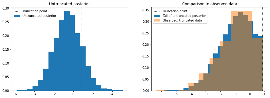
[28]:
f, axes = plt.subplots(1, 2, figsize=(15, 5))

axes[0].hist(
    samples_thinned.copy(), label="Untruncated posterior", bins=20, density=True
)
axes[0].axvline(true_high, linestyle=":", color="k", label="Truncation point")
axes[0].set_title("Untruncated posterior")
axes[0].legend()

axes[1].hist(
    samples_thinned[samples_thinned < true_high].copy(),
    label="Tail of untruncated posterior",
    bins=20,
    density=True,
)
axes[1].hist(true_x.copy(), label="Observed, truncated data", density=True, alpha=0.5)
axes[1].axvline(true_high, linestyle=":", color="k", label="Truncation point")
axes[1].set_title("Comparison to observed data")
axes[1].legend()
plt.show()
5.3 示例:左截断泊松分布
作为最后一个示例,我们现在实现一个左截断泊松分布。请注意,右截断泊松分布可以被重构为分类分布的一个特例,因此我们关注不那么平凡的情况。
类属性
对于截断泊松分布,我们需要两个参数:原始泊松分布的 rate 和一个指示截断点的 low 参数。由于这是一个离散分布,我们需要明确截断点是否包含在支撑集中。在本教程中,我们约定截断点 low 是支撑集的一部分。
low 参数必须给定“非负整数”约束。由于它是一个离散参数,使用 NUTS 对此参数进行推断是不可能的。这很可能不是问题,因为截断点通常是预先知道的。然而,如果确实需要推断 low 参数,可以使用 DiscreteHMCGibbs 来实现,尽管只能使用具有枚举支撑集的先验。
与截断正态分布的情况类似,此分布的支撑集将定义为属性而非类属性,因为它取决于 low 参数的具体值。
class LeftTruncatedPoisson:
    arg_constraints = {
        "low": constraints.nonnegative_integer,
        "rate": constraints.positive,
    }

    # ...
    @constraints.dependent_property(is_discrete=True)
    def support(self):
        return constraints.integer_greater_than(self.low - 1)
在 dependent_property 装饰器中传递的 is_discrete 参数用于告诉推断算法哪些变量是离散隐变量。
__init__ 方法
这里我们遵循与前一个示例相同的模式。
# ...
def __init__(self, rate=1.0, low=0, validate_args=None):
    batch_shape = lax.broadcast_shapes(
        jnp.shape(low), jnp.shape(rate)
    )
    self.low, self.rate = promote_shapes(low, rate)
    super().__init__(batch_shape, validate_args=validate_args)
# ...
log_prob 方法
逻辑与截断正态分布情况非常相似。但这次我们是在左侧截断,因此正确的归一化是互补累积密度
对于代码,我们可以依赖 jax.scipy.stats 中的 poisson 模块。
# ...
def log_prob(self, value):
    m = 1 - poisson.cdf(self.low - 1, self.rate)
    log_p = poisson.logpmf(value, self.rate)
    return jnp.where(value >= self.low, log_p - jnp.log(m), -jnp.inf)
# ...
sample 方法
逆变换采样也适用于离散分布。离散分布的“逆”CDF 定义为
或者,用通俗的话讲,\(F^{-1}(u)\) 是累积密度小于 \(u\) 的最大数字。然而,目前 Jax 中还没有泊松分布 \(F^{-1}\) 的实现(至少在编写本教程时如此)。我们必须依赖自己的实现。幸运的是,我们可以利用离散分布的特性,轻松实现一个“暴力”版本,该版本适用于大多数情况。暴力方法包括简单地按顺序扫描所有非负整数,一个接一个,直到累积密度的值超过参数 \(u\)。隐性要求是我们有办法评估截断分布的累积密度,但这我们可以计算得到
当然,如果 \(z < L\),\(F_Z(z)\) 的值为零。(与前一个示例一样,我们使用 \(Y\) 表示原始、未截断的变量,使用 \(Z\) 表示截断的变量)
# ...
def sample(self, key, sample_shape=()):
    shape = sample_shape + self.batch_shape
    minval = jnp.finfo(jnp.result_type(float)).tiny
    u = random.uniform(key, shape, minval=minval)
    return self.icdf(u)

def icdf(self, u):
    def cond_fn(val):
        n, cdf = val
        return jnp.any(cdf < u)

    def body_fn(val):
        n, cdf = val
        n_new = jnp.where(cdf < u, n + 1, n)
        return n_new, self.cdf(n_new)

    low = self.low * jnp.ones_like(u)
    cdf = self.cdf(low)
    n, _ = lax.while_loop(cond_fn, body_fn, (low, cdf))
    return n.astype(jnp.result_type(int))

def cdf(self, value):
    m = 1 - poisson.cdf(self.low - 1, self.rate)
    f = poisson.cdf(value, self.rate) - poisson.cdf(self.low - 1, self.rate)
    return jnp.where(k >= self.low, f / m, 0)
关于上述实现的几点说明
即使使用双精度,如果
rate远小于low,上述代码也将无法工作。由于数值限制,会得到poisson.cdf(low - 1, rate)等于(或非常接近)1.0。这将导致无法准确地重新加权分布,因为归一化常数将为0.0。暴力
icdf方法当然非常慢,特别是在rate很高时。如果需要更快的采样,一种选择是依赖更快的搜索算法。例如
def icdf_faster(self, u):
    num_bins = 200 # Choose a reasonably large value
    bins = jnp.arange(num_bins)
    cdf = self.cdf(bins)
    indices = jnp.searchsorted(cdf, u)
    return bins[indices]
这里明显的限制是 bin 的数量必须预先固定(jax 不允许动态大小的数组)。另一个选择是依赖于本文中提出的近似实现。
对于
icdf,另一种替代方法是依赖scipy的实现并使用 Jax 的host_callback模块。此功能允许您使用 Python 函数,而无需在Jax中编写代码。这意味着我们可以简单地使用scipy对泊松 ICDF 的实现!从最后一个等式,我们可以写出截断的 icdf 为
在 python 中
def scipy_truncated_poisson_icdf(args): # Note: all arguments are passed inside a tuple
    rate, low, u = args
    rate = np.asarray(rate)
    low = np.asarray(low)
    u = np.asarray(u)
    density = sp_poisson(rate)
    low_cdf = density.cdf(low - 1)
    normalizer = 1.0 - low_cdf
    x = normalizer * u + low_cdf
    return density.ppf(x)
原则上,在我们的 NumPyro 分布中无法使用上述函数,因为它不是用 Jax 编写的。jax.experimental.host_callback.call 函数正好解决了这个问题。下面的代码展示了如何使用它,但请记住,这目前是一个实验性功能,因此该模块可能会发生变化。更多详细信息请参阅 host_callback 文档。
# ...
def icdf_scipy(self, u):
    result_shape = jax.ShapeDtypeStruct(
        u.shape,
        jnp.result_type(float) # int type not currently supported
    )
    result = jax.experimental.host_callback.call(
        scipy_truncated_poisson_icdf,
        (self.rate, self.low, u),
        result_shape=result_shape
    )
    return result.astype(jnp.result_type(int))
# ...
综合起来,实现如下所示
[29]:
def scipy_truncated_poisson_icdf(args):  # Note: all arguments are passed inside a tuple
    rate, low, u = args
    rate = np.asarray(rate)
    low = np.asarray(low)
    u = np.asarray(u)
    density = sp_poisson(rate)
    low_cdf = density.cdf(low - 1)
    normalizer = 1.0 - low_cdf
    x = normalizer * u + low_cdf
    return density.ppf(x)


class LeftTruncatedPoisson(Distribution):
    """
    A truncated Poisson distribution.
    :param numpy.ndarray low: lower bound at which truncation happens
    :param numpy.ndarray rate: rate of the Poisson distribution.
    """

    arg_constraints = {
        "low": constraints.nonnegative_integer,
        "rate": constraints.positive,
    }

    def __init__(self, rate=1.0, low=0, validate_args=None):
        batch_shape = lax.broadcast_shapes(jnp.shape(low), jnp.shape(rate))
        self.low, self.rate = promote_shapes(low, rate)
        super().__init__(batch_shape, validate_args=validate_args)

    def log_prob(self, value):
        m = 1 - poisson.cdf(self.low - 1, self.rate)
        log_p = poisson.logpmf(value, self.rate)
        return jnp.where(value >= self.low, log_p - jnp.log(m), -jnp.inf)

    def sample(self, key, sample_shape=()):
        shape = sample_shape + self.batch_shape
        float_type = jnp.result_type(float)
        minval = jnp.finfo(float_type).tiny
        u = random.uniform(key, shape, minval=minval)
        # return self.icdf(u)        # Brute force
        # return self.icdf_faster(u) # For faster sampling.
        return self.icdf_scipy(u)  # Using `host_callback`

    def icdf(self, u):
        def cond_fn(val):
            n, cdf = val
            return jnp.any(cdf < u)

        def body_fn(val):
            n, cdf = val
            n_new = jnp.where(cdf < u, n + 1, n)
            return n_new, self.cdf(n_new)

        low = self.low * jnp.ones_like(u)
        cdf = self.cdf(low)
        n, _ = lax.while_loop(cond_fn, body_fn, (low, cdf))
        return n.astype(jnp.result_type(int))

    def icdf_faster(self, u):
        num_bins = 200  # Choose a reasonably large value
        bins = jnp.arange(num_bins)
        cdf = self.cdf(bins)
        indices = jnp.searchsorted(cdf, u)
        return bins[indices]

    def icdf_scipy(self, u):
        result_shape = jax.ShapeDtypeStruct(u.shape, jnp.result_type(float))
        result = jax.experimental.host_callback.call(
            scipy_truncated_poisson_icdf,
            (self.rate, self.low, u),
            result_shape=result_shape,
        )
        return result.astype(jnp.result_type(int))

    def cdf(self, value):
        m = 1 - poisson.cdf(self.low - 1, self.rate)
        f = poisson.cdf(value, self.rate) - poisson.cdf(self.low - 1, self.rate)
        return jnp.where(value >= self.low, f / m, 0)

    @constraints.dependent_property(is_discrete=True)
    def support(self):
        return constraints.integer_greater_than(self.low - 1)
试试看!
[30]:
def discrete_distplot(samples, ax=None, **kwargs):
    """
    Utility function for plotting the samples as a barplot.
    """
    x, y = np.unique(samples, return_counts=True)
    y = y / sum(y)
    if ax is None:
        ax = plt.gca()

    ax.bar(x, y, **kwargs)
    return ax
[31]:
def truncated_poisson_model(num_observations, x=None):
    low = numpyro.sample("low", dist.Categorical(0.2 * jnp.ones((5,))))
    rate = numpyro.sample("rate", dist.LogNormal(1, 1))
    with numpyro.plate("observations", num_observations):
        numpyro.sample("x", LeftTruncatedPoisson(rate, low), obs=x)
先验样本
[32]:
# -- prior samples
num_observations = 1000
num_prior_samples = 100
prior = Predictive(truncated_poisson_model, num_samples=num_prior_samples)
prior_samples = prior(PRIOR_RNG, num_observations)
推断
与截断正态分布的情况一样,这里最好替换 low 参数上的先验,使其与观测数据一致。我们希望在 low 上有一个分类先验(这样我们可以使用 DiscreteHMCGibbs),其最高类别等于 x 的最小值(这样先验和数据一致)。然而,在编写此类模型时必须小心,因为 Jax 不允许动态大小的数组。编写此模型的一个简单方法是仅将类别数指定为一个参数
[33]:
def truncated_poisson_model(num_observations, x=None, k=5):
    zeros = jnp.zeros((k,))
    low = numpyro.sample("low", dist.Categorical(logits=zeros))
    rate = numpyro.sample("rate", dist.LogNormal(1, 1))
    with numpyro.plate("observations", num_observations):
        numpyro.sample("x", LeftTruncatedPoisson(rate, low), obs=x)
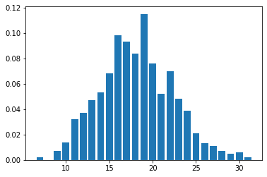
[34]:
# Take any prior sample as the true process.
true_idx = 6
true_low = prior_samples["low"][true_idx]
true_rate = prior_samples["rate"][true_idx]
true_x = prior_samples["x"][true_idx]
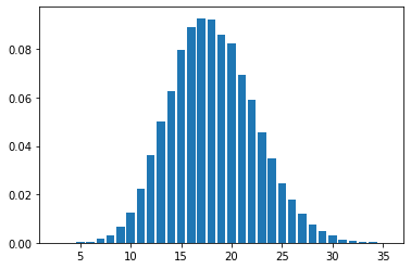
discrete_distplot(true_x.copy());
为了进行推断,我们将 k = x.min() + 1。另请注意使用 DiscreteHMCGibbs
[35]:
mcmc = MCMC(DiscreteHMCGibbs(NUTS(truncated_poisson_model)), **MCMC_KWARGS)
mcmc.run(MCMC_RNG, num_observations, true_x, k=true_x.min() + 1)
mcmc.print_summary()
sample: 100%|██████████████████████████████████████████████████████████████████████████████████████████████████████████████████████████| 4000/4000 [00:04<00:00, 808.70it/s, 3 steps of size 9.58e-01. acc. prob=0.93]
sample: 100%|█████████████████████████████████████████████████████████████████████████████████████████████████████████████████████████| 4000/4000 [00:00<00:00, 5916.30it/s, 3 steps of size 9.14e-01. acc. prob=0.93]
sample: 100%|█████████████████████████████████████████████████████████████████████████████████████████████████████████████████████████| 4000/4000 [00:00<00:00, 5082.16it/s, 3 steps of size 9.91e-01. acc. prob=0.92]
sample: 100%|█████████████████████████████████████████████████████████████████████████████████████████████████████████████████████████| 4000/4000 [00:00<00:00, 6511.68it/s, 3 steps of size 8.66e-01. acc. prob=0.94]
                mean       std    median      5.0%     95.0%     n_eff     r_hat
       low      4.13      2.43      4.00      0.00      7.00   7433.79      1.00
      rate     18.16      0.14     18.16     17.96     18.40   3074.46      1.00
[36]:
true_rate
[36]:
DeviceArray(18.2091848, dtype=float64)
如前所述,在估计截断点时需要格外小心。如果截断点已知,最好提供它。
[37]:
model_with_known_low = numpyro.handlers.condition(
    truncated_poisson_model, {"low": true_low}
)
另请注意,我们可以直接使用 NUTS,因为无需推断任何离散参数。
[38]:
mcmc = MCMC(
    NUTS(model_with_known_low),
    **MCMC_KWARGS,
)
[39]:
mcmc.run(MCMC_RNG, num_observations, true_x)
mcmc.print_summary()
sample: 100%|█████████████████████████████████████████████████████████████████████████████████████████████████████████████████████████| 4000/4000 [00:03<00:00, 1185.13it/s, 1 steps of size 9.18e-01. acc. prob=0.93]
sample: 100%|█████████████████████████████████████████████████████████████████████████████████████████████████████████████████████████| 4000/4000 [00:00<00:00, 5786.32it/s, 3 steps of size 1.00e+00. acc. prob=0.92]
sample: 100%|█████████████████████████████████████████████████████████████████████████████████████████████████████████████████████████| 4000/4000 [00:00<00:00, 5919.13it/s, 1 steps of size 8.62e-01. acc. prob=0.94]
sample: 100%|█████████████████████████████████████████████████████████████████████████████████████████████████████████████████████████| 4000/4000 [00:00<00:00, 7562.36it/s, 3 steps of size 9.01e-01. acc. prob=0.93]
                mean       std    median      5.0%     95.0%     n_eff     r_hat
      rate     18.17      0.13     18.17     17.95     18.39   3406.81      1.00

Number of divergences: 0
移除截断
[40]:
model_without_truncation = numpyro.handlers.condition(
    truncated_poisson_model,
    {"low": 0},
)
pred = Predictive(model_without_truncation, posterior_samples=mcmc.get_samples())
pred_samples = pred(PRED_RNG, num_observations)
thinned_samples = pred_samples["x"][::500]
[41]:
discrete_distplot(thinned_samples.copy());