求解多初始条件的常微分方程 (ODEs)。
常微分方程 (ODEs) 在流行病学、物理、化学、金融等各种领域都有应用。通常,ODE 系统需要在保持参数不变的情况下对多个初始条件进行积分。此外,典型数据集通常包含缺失值、表现出不同的持续时间并且具有不规则间隔的数据点。本教程在前一个捕食者-猎物模型 教程 的基础上,解决了这些挑战。我们将
定义 ODE 和概率模型。
生成带瑕疵的合成数据集。
使用 MCMC 算法执行参数估计。
[ ]:
#!pip install -q numpyro@git+https://github.com/pyro-ppl/numpyro
[2]:
import functools

import matplotlib.pyplot as plt

import jax
from jax.experimental.ode import odeint
import jax.numpy as jnp
from jax.random import PRNGKey

import numpyro
import numpyro.distributions as dist
from numpyro.infer import MCMC, NUTS, Predictive, init_to_sample

# Numerical instabilities may arise during ODE solving,
# so one has sometimes to play around with solver settings,
# change solver, or change numeric precision as we do here.
numpyro.enable_x64(True)
模型
首先,我们定义微分方程 dz_dt 和概率模型 model。微分方程与 Lotka-Volterra 教程中的相同。然而,模型中引入了显着的变化,以同时适应多个初始条件。我们首先采样初始条件 z_init 和参数 theta。接着,以向量化形式求解 ODE 系统。使用 jax.vmap 并结合 functools.partial 传递 kwargs 来实现向量化。然后,我们采样 sigma 来表示测量误差。最后,我们采样测量的种群。考虑到观测到的 y 中可能存在缺失值,我们对非有限值进行掩码处理。
[3]:
def dz_dt(z, t, theta):
    """
    Lotka–Volterra equations. Real positive parameters `alpha`, `beta`, `gamma`, `delta`
    describes the interaction of two species.
    """
    u, v = z
    alpha, beta, gamma, delta = theta

    du_dt = (alpha - beta * v) * u
    dv_dt = (-gamma + delta * u) * v
    return jnp.stack([du_dt, dv_dt])


def model(ts, y_init, y=None):
    """
    :param numpy.ndarray ts: measurement times
    :param numpy.ndarray y_init: measured inital conditions
    :param numpy.ndarray y: measured populations
    """
    # initial population
    z_init = numpyro.sample(
        "z_init", dist.LogNormal(jnp.log(y_init), jnp.ones_like(y_init))
    )

    # parameters alpha, beta, gamma, delta of dz_dt
    theta = numpyro.sample(
        "theta",
        dist.TruncatedNormal(
            low=0.0,
            loc=jnp.array([1.0, 0.05, 1.0, 0.05]),
            scale=jnp.array([0.2, 0.01, 0.2, 0.01]),
        ),
    )

    # helpers to solve ODEs in a vectorized form
    odeint_with_kwargs = functools.partial(odeint, rtol=1e-6, atol=1e-5, mxstep=1000)
    vect_solve_ode = jax.vmap(
        odeint_with_kwargs,
        in_axes=(None, 0, 0, None),
    )

    # integrate dz/dt
    zs = vect_solve_ode(dz_dt, z_init, ts, theta)
    # measurement errors
    sigma = numpyro.sample("sigma", dist.LogNormal(-1, 1).expand([2]))
    # measured populations
    if y is not None:
        # mask missing observations in the observed y
        mask = jnp.isfinite(jnp.log(y))
        numpyro.sample("y", dist.LogNormal(jnp.log(zs), sigma).mask(mask), obs=y)
    else:
        numpyro.sample("y", dist.LogNormal(jnp.log(zs), sigma))
数据集
为了本教程的目的,我们将利用从先前定义的模型中采样生成的合成数据集。为了模拟实际数据集的非理想特性,我们将引入缺失值、变化的持续时间以及时间点之间的不规则间隔。需要注意的是,JAX 使用向量化和编译计算,要求数据集具有相同的长度。在本例中,尽管我们有不同的间隔,但点数保持相同。如果点数不同,可以使用 jnp.pad 将所有数据集扩展到相同长度,并填充虚拟值,这些虚拟值之后可以被掩码忽略。
首先,让我们建立模拟设置。数据集的时间跨度将在 t_min 和 t_max 之间变化,点数限制在 n_points_min 和 n_points_max 之间。此外,我们将以概率 p_missing 引入缺失值。
[4]:
n_datasets = 3  # int n_datasets: number of datasets to generate
t_min = 100  # int t_min: minimal allowed length of the generated time array
t_max = 200  # int t_min: maximal allowed length of the generated time array
n_points_min = 80  # int n_points_min: minimal allowed number of points in a data set
n_points_max = 120  # int n_points_max: maximal allowed number of points in a data set
y0_min = 2.0  # float y0_min: minimal allowed value for initial conditions
y0_max = 10.0  # float y0_max: maximal allowed value for initial conditions
p_missing = 0.1  # float p_missing: probability of having missing values
生成包含初始条件的数组
[5]:
# generate an array with initial conditons
z_inits = jnp.array(
    [jnp.linspace(y0_min, y0_max, n_datasets), jnp.linspace(y0_max, y0_min, n_datasets)]
).T

print(f"Initial conditons are: \n {z_inits}")
Initial conditons are:
 [[ 2. 10.]
 [ 6.  6.]
 [10.  2.]]
接下来,我们创建一个时间矩阵 ts,用于存储每个单独数据集的时间点。我们将在 rand_duration 中生成 t_min 和 t_max 之间的随机整数,以表示变化的持续时间。类似地,rand_n_points 将对应于每个数据集中的不同间隔。由于 JAX 需要一个具有恒定形状的矩阵,我们将使用 jnp.pad 将单个观测填充到最长数组的共同长度。
[6]:
# generate array with random integers between t_min and t_max, representing tiem duration in the data set
rand_duration = jax.random.randint(
    PRNGKey(1), shape=(n_datasets,), minval=t_min, maxval=t_max
)

# generate array with random integers between n_points_min and n_points_max,
# representing number of time points per dataset
rand_n_points = jax.random.randint(
    PRNGKey(1), shape=(n_datasets,), minval=n_points_min, maxval=n_points_max
)

# Note that arrays have different length and are stored in a list
time_arrays = [
    jnp.linspace(0, j, num=rand_n_points[i]).astype(float)
    for i, j in enumerate(rand_duration)
]
longest = jnp.max(jnp.array([len(i) for i in time_arrays]))

# Make a time matrix
ts = jnp.array(
    [
        jnp.pad(arr, pad_width=(0, longest - len(arr)), constant_values=jnp.nan)
        for arr in time_arrays
    ]
)

print(f"The shape of the time matrix is {ts.shape}")
print(f"First values are \n {ts[:, :10]}")
print(f"Last values are \n {ts[:, -10:]}")
The shape of the time matrix is (3, 108)
First values are
 [[ 0.          1.00934579  2.01869159  3.02803738  4.03738318  5.04672897
   6.05607477  7.06542056  8.07476636  9.08411215]
 [ 0.          1.23863636  2.47727273  3.71590909  4.95454545  6.19318182
   7.43181818  8.67045455  9.90909091 11.14772727]
 [ 0.          1.21212121  2.42424242  3.63636364  4.84848485  6.06060606
   7.27272727  8.48484848  9.6969697  10.90909091]]
Last values are
 [[ 98.91588785  99.92523364 100.93457944 101.94392523 102.95327103
  103.96261682 104.97196262 105.98130841 106.99065421 108.        ]
 [         nan          nan          nan          nan          nan
           nan          nan          nan          nan          nan]
 [118.78787879 120.                  nan          nan          nan
           nan          nan          nan          nan          nan]]
我们将利用 NumPyro 的 Predictive 模式抽取单个样本,代表我们的合成数据集。随后,我们将对数据应用一个带有 NaNs 的掩码,以模拟缺失值。为简单起见,我们将确保初始值不缺失。在实际数据集中这可能不成立,这时可以应用各种填充方法。
[7]:
# take a single sample that will be our synthetic data
sample = Predictive(model, num_samples=1)(PRNGKey(100), ts, z_inits)
data = sample["y"][0]

# create a mask that will add missing values to the data
missing_obs_mask = jax.random.choice(
    PRNGKey(1),
    jnp.array([True, False]),
    shape=data.shape,
    p=jnp.array([p_missing, 1 - p_missing]),
)
# make sure that initial values are not missing
missing_obs_mask = missing_obs_mask.at[:, 0, :].set(False)

# data with missing values
data = data.at[missing_obs_mask].set(jnp.nan)
最后,为了后续与 NUTS 兼容,我们需要用虚拟变量填充时间矩阵 ts 中的 NaN 值。JAX 的 odeint 函数要求这些值是递增的。我们用时间矩阵中大于 t_max 的值填充它们。重要的是,这些值不影响 MCMC 估计,因为 data 中相应的值是缺失的,因此在后验估计期间会被忽略。
[8]:
# fill_nans
def fill_nans(ts):
    n_nan = jnp.sum(jnp.isnan(ts))
    if n_nan > 0:
        loc_first_nan = jnp.where(jnp.isnan(ts))[0][0]
        ts_filled_nans = ts.at[loc_first_nan:].set(
            jnp.linspace(t_max, t_max + 20, n_nan)
        )
        return ts_filled_nans
    else:
        return ts


ts_filled_nans = jnp.array([fill_nans(t) for t in ts])
我们来简要总结一下我们的合成数据集
[9]:
print(f"The dataset has the shape {data.shape}, (n_datasets, n_points, n_observables)")
print(f"The time matrix has the shape {ts.shape}, (n_datasets, n_timepoints)")
print(f"The time matrix has different spacing between timepoints: \n {ts[:, :5]}")
print(f"The final timepoints are: {jnp.nanmax(ts, 1)} years.")
print(
    f"The dataset has {jnp.sum(jnp.isnan(data)) / jnp.size(data):.0%} missing observations"
)
print(f"True params mean: {sample['theta'][0]}")
The dataset has the shape (3, 108, 2), (n_datasets, n_points, n_observables)
The time matrix has the shape (3, 108), (n_datasets, n_timepoints)
The time matrix has different spacing between timepoints:
 [[0.         1.00934579 2.01869159 3.02803738 4.03738318]
 [0.         1.23863636 2.47727273 3.71590909 4.95454545]
 [0.         1.21212121 2.42424242 3.63636364 4.84848485]]
The final timepoints are: [108. 109. 120.] years.
The dataset has 19% missing observations
True params mean: [0.78770691 0.05049109 0.89073622 0.05296055]
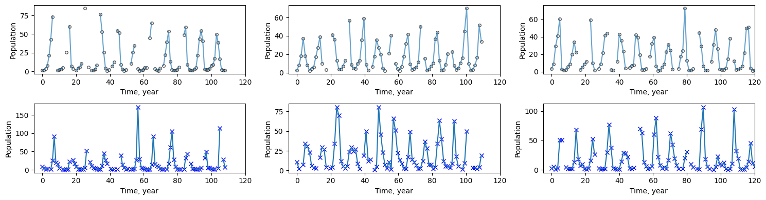
让我们可视化数据集,用实线帮助引导眼睛。您会注意到 NaN 值出现的地方有断线。
[10]:
# Plotting
fig, axs = plt.subplots(2, n_datasets, figsize=(15, 4))

for i in range(n_datasets):
    loc = jnp.where(jnp.isfinite(data[i, :, 0]))[0][-1]

    axs[0, i].plot(
        ts[i, :], data[i, :, 0], "ko", mfc="none", ms=4, label="true hare", alpha=0.67
    )
    axs[0, i].plot(ts[i, :], data[i, :, 0], label="true hare", alpha=0.67)
    axs[0, i].set_xlabel("Time, year")
    axs[0, i].set_ylabel("Population")
    axs[0, i].set_xlim([-5, jnp.nanmax(ts)])

    axs[1, i].plot(ts[i, :], data[i, :, 1], "bx", label="true lynx")
    axs[1, i].plot(ts[i, :], data[i, :, 1], label="true lynx")
    axs[1, i].set_xlabel("Time, year")
    axs[1, i].set_ylabel("Population")
    axs[1, i].set_xlim([-5, jnp.nanmax(ts)])

fig.tight_layout()
执行 MCMC。
为了在准确性和速度之间取得平衡,必须调整 MCMC 求解器和 ODE 求解器的参数以适应具体问题。
[11]:
y_init = data[:, 0, :]

mcmc = MCMC(
    NUTS(
        model,
        dense_mass=True,
        init_strategy=init_to_sample(),
        max_tree_depth=10,
    ),
    num_warmup=1000,
    num_samples=1000,
    num_chains=1,
    progress_bar=True,
)

mcmc.run(PRNGKey(1031410), ts=ts_filled_nans, y_init=y_init, y=data)
mcmc.print_summary()

print(f"True params mean: {sample['theta'][0]}")
print(f"Estimated params mean: {jnp.mean(mcmc.get_samples()['theta'], axis=0)}")
sample: 100%|██████████| 2000/2000 [09:09<00:00, 3.64it/s, 31 steps of size 1.23e-01. acc. prob=0.94]
                 mean       std    median      5.0%     95.0%     n_eff     r_hat
   sigma[0]      0.29      0.01      0.29      0.27      0.31   1064.77      1.00
   sigma[1]      0.51      0.02      0.51      0.47      0.55   1593.43      1.00
   theta[0]      0.77      0.02      0.77      0.74      0.79    760.41      1.00
   theta[1]      0.05      0.00      0.05      0.05      0.05    888.74      1.00
   theta[2]      0.91      0.02      0.91      0.87      0.94    842.09      1.00
   theta[3]      0.06      0.00      0.06      0.05      0.06    858.84      1.00
z_init[0,0]      1.51      0.05      1.51      1.43      1.60    782.07      1.00
z_init[0,1]      9.11      0.55      9.09      8.06      9.88   1072.88      1.00
z_init[1,0]      3.83      0.14      3.83      3.63      4.07    986.01      1.00
z_init[1,1]      8.54      0.57      8.54      7.66      9.52    945.91      1.00
z_init[2,0]      3.87      0.15      3.86      3.64      4.11   1210.24      1.00
z_init[2,1]      3.70      0.19      3.69      3.39      4.02   1342.93      1.00

Number of divergences: 0
True params mean: [0.78770691 0.05049109 0.89073622 0.05296055]
Estimated params mean: [0.7684689  0.05000161 0.90749349 0.05559383]
运行预测。
[12]:
# predict
ts_pred = jnp.tile(jnp.linspace(0, 200, 1000), (n_datasets, 1))
pop_pred = Predictive(model, mcmc.get_samples())(PRNGKey(1041140), ts_pred, y_init)["y"]
mu = jnp.mean(pop_pred, 0)
pi = jnp.percentile(pop_pred, jnp.array([10, 90]), 0)


print(f"True params mean: {sample['theta'][0]}")
print(f"Estimated params mean: {jnp.mean(mcmc.get_samples()['theta'], axis=0)}")
True params mean: [0.78770691 0.05049109 0.89073622 0.05296055]
Estimated params mean: [0.7684689  0.05000161 0.90749349 0.05559383]
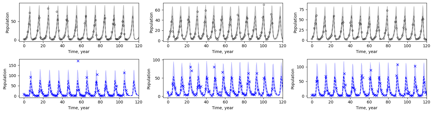
绘制观测点、预测均值及预测区间。
[13]:
# Plotting
fig, axs = plt.subplots(2, n_datasets, figsize=(15, 4))

for i in range(n_datasets):
    loc = jnp.where(jnp.isfinite(data[i, :, 0]))[0][-1]

    axs[0, i].plot(
        ts_pred[i, :], mu[i, :, 0], "k-.", label="pred hare", lw=1, alpha=0.67
    )
    axs[0, i].plot(
        ts[i, :], data[i, :, 0], "ko", mfc="none", ms=4, label="true hare", alpha=0.67
    )
    axs[0, i].fill_between(
        ts_pred[i, :], pi[0, i, :, 0], pi[1, i, :, 0], color="k", alpha=0.2
    )
    axs[0, i].set_xlabel("Time, year")
    axs[0, i].set_ylabel("Population")
    axs[0, i].set_xlim([-5, jnp.nanmax(ts)])

    axs[1, i].plot(ts_pred[i, :], mu[i, :, 1], "b--", label="pred lynx")
    axs[1, i].plot(ts[i, :], data[i, :, 1], "bx", label="true lynx")
    axs[1, i].fill_between(
        ts_pred[i, :], pi[0, i, :, 1], pi[1, i, :, 1], color="b", alpha=0.2
    )
    axs[1, i].set_xlabel("Time, year")
    axs[1, i].set_ylabel("Population")
    axs[1, i].set_xlim([-5, jnp.nanmax(ts)])


fig.tight_layout()