示例:高斯过程的希尔伯特空间近似(多维)
高斯过程模型(参见 示例:高斯过程)是一类灵活的模型,可用于回归、分类和无监督学习。由于它们的缩放性能较差,不适用于大型数据集。希尔伯特空间近似(参见 示例:高斯过程的希尔伯特空间近似)提供了一种可扩展的替代方案。本示例将前一个示例中研究的单变量情况扩展到多维输入情况,并演示了 贡献的 HSGP 模块 的使用。
首先,加载所需的库并配置 jax 和 numpyro。
[1]:
#!pip install -q numpyro@git+https://github.com/pyro-ppl/numpyro
[2]:
from typing import Sequence

import arviz as az
import matplotlib.pyplot as plt
import numpy as np
from numpy.typing import NDArray

import jax
from jax import random
import jax.numpy as jnp
from optax import linear_onecycle_schedule

import numpyro
from numpyro import distributions as dist
from numpyro.contrib.hsgp.approximation import hsgp_squared_exponential
from numpyro.infer import Predictive
from numpyro.infer.autoguide import AutoNormal
from numpyro.infer.elbo import Trace_ELBO
from numpyro.infer.hmc import NUTS
from numpyro.infer.initialization import init_to_median, init_to_uniform
from numpyro.infer.mcmc import MCMC
from numpyro.infer.svi import SVI
from numpyro.optim import Adam
[3]:
num_devices = 4
numpyro.set_host_device_count(num_devices)
jax.config.update(
    "jax_enable_x64", True
)  # additional precision for to avoid numerical issues with Cholesky decomposition of the covariance matrix
绘制模拟数据
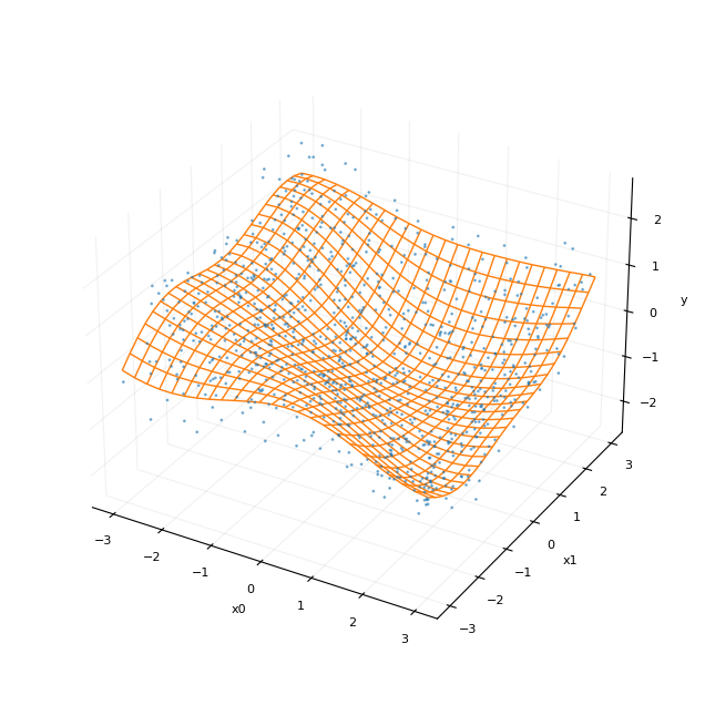
首先,我们从一个具有平方指数核函数(squared exponential kernel function)的 D 维高斯过程中采样 N 个点。输入点从覆盖域 \([-L, L]^D\) 的正方形/超立方体上的均匀分布中抽取。我们还从均匀间隔的输入网格中采样一组(无噪声)点,以便可视化生成过程。由于我们的模型假设高斯过程是中心化的,因此在返回输出空间中的点之前,我们会对其进行去均值处理。sample_grid_and_data 函数返回网格化值和数据点。se_kernel 函数实现了高斯过程的协方差函数。
[4]:
def se_kernel(
    X: jax.Array,
    Z: jax.Array,
    amplitude: float,
    length: float,
    noise: float | None,
    jitter=1.0e-6,
) -> jax.Array:
    """Squared exponential kernel function."""
    r = jnp.linalg.norm(X[:, jnp.newaxis] - Z, axis=-1)
    delta = (r / length) ** 2
    k = (amplitude**2) * jnp.exp(-0.5 * delta)
    if noise is None:
        return k
    else:
        return k + (noise**2 + jitter) * jnp.eye(k.shape[0])


def sample_grid_and_data(
    N_grid: int,
    N: int,
    L: float,
    amplitude: float,
    lengthscale: float,
    noise: float,
    key: int,
    D: int,
) -> tuple[jax.Array, jax.Array, jax.Array, jax.Array]:
    """Sample N_grid ** D points from noiseless function and N noisy data points from a GP."""

    # draw points on a grid for plotting surface of the noiseless function
    x_linspace = jnp.linspace(-L, L, N_grid)
    x_mesh = jnp.meshgrid(*[x_linspace for _ in range(D)])
    X_grid = jnp.concatenate([x_mesh[i].ravel()[..., None] for i in range(D)], axis=1)

    # draw data points from a uniform distribution on the support of the grid
    X = random.uniform(key, shape=(N, D), minval=-L, maxval=L)

    # concatenate grid and data points
    X_all = jnp.concatenate([X_grid, X], axis=0)

    # sample from the GP
    cov = se_kernel(X_all, X_all, amplitude, lengthscale, 0.0)  # noiseless
    _, key = random.split(key)
    _y = random.multivariate_normal(key, mean=jnp.zeros(cov.shape[0]), cov=cov)

    # separate the grid and data points
    y_grid = _y[0 : N_grid**D].reshape((N_grid,) * D)
    _, key = random.split(key)
    y = _y[N_grid**D :] + (
        random.normal(key, shape=(N,)) * noise
    )  # add noise to the data points

    y_mean = y.mean()

    return X_grid, y_grid - y_mean, X, y - y_mean
本示例中我们将 D=2 固定,但代码是完全通用的。将渲染一维和二维情况下的图。我们将 N=1000 和 L=3.0。
[5]:
# parameters for the synthetic data
D = 2
N_grid = 25 if D == 2 else 100
N = 1_000
L = 3.0

# kernel parameters
amplitude = 1.0
lengthscale = 2.0

# noise level
noise = 0.5 if D == 2 else 0.15

# sample the grid and data
seed = 0
key = jax.random.key(seed)

X_grid, y_grid, X, y = sample_grid_and_data(
    N_grid, N, L, amplitude, lengthscale, noise, key, D
)
在进行建模之前,我们将设置一些绘图函数,以帮助可视化生成过程和后验预测分布。我们将在二维情况下使用 plot_surface_scatter,在一维情况下使用 plot_line_scatter。
[6]:
def plot_surface_scatter(
    N_grid: int,
    X_grid: NDArray | None = None,
    y_grid: NDArray | None = None,
    X: NDArray | None = None,
    y: NDArray | None = None,
    test_ind: jax.Array | None = None,
    post_y: jax.Array | None = None,
    xz_lines: list[tuple[jax.Array, jax.Array, float]] | None = None,
    yz_lines: list[tuple[jax.Array, jax.Array, float]] | None = None,
    xy_annotate_lines: Sequence[
        tuple[tuple[float, float], tuple[float, float]] | None
    ] = None,
    fig_size: float = 8.0,
    label_size: float = 8.0,
    grid_alpha: float = 0.1,
    y_wireframe_alpha: float = 1.0,
    post_alpha: float = 0.1,
    point_size: float = 1.0,
    point_alpha: float = 0.5,
    ci_alpha: float = 0.1,
) -> None:
    # setup figure
    fig = plt.figure(figsize=(fig_size, fig_size))

    # plot the surface of the noiseless function and the data points
    x0_grid, x1_grid = (
        X_grid[:, 0].reshape((N_grid, N_grid)),
        X_grid[:, 1].reshape((N_grid, N_grid)),
    )
    ax = fig.add_subplot(projection="3d")

    # plot wireframes from draws from the posterior
    if post_y is not None:
        for i in range(post_y.shape[0]):
            post_y_grid = post_y[i, :].reshape((N_grid, N_grid))
            ax.plot_wireframe(
                x0_grid,
                x1_grid,
                post_y_grid,
                rstride=1,
                cstride=1,
                linewidth=1.0,
                alpha=post_alpha,
                color="tab:blue",
            )

    # plot the data points
    if X is not None and y is not None:
        color = (
            "tab:blue"
            if test_ind is None
            else np.where(test_ind, "tab:green", "tab:blue")
        )
        ax.scatter(
            xs=X[:, 0],
            ys=X[:, 1],
            zs=y,
            c=color,
            s=point_size,
            alpha=point_alpha,
        )

    # add confidence intervals at the boundaries
    if xz_lines:
        for line in xz_lines:
            x, z, y = line
            ax.plot(
                x, z, zs=y, zdir="y", color="tab:green", linestyle="--", alpha=ci_alpha
            )
    if yz_lines:
        for line in yz_lines:
            y, z, x = line
            ax.plot(
                y, z, zs=x, zdir="x", color="tab:green", linestyle="--", alpha=ci_alpha
            )

    # plot the surface of the noiseless function
    if y_grid is not None:
        ax.plot_wireframe(
            x0_grid,
            x1_grid,
            y_grid,
            rstride=1,
            cstride=1,
            linewidths=1.0,
            alpha=y_wireframe_alpha,
            color="tab:orange",
        )

    # add box in xy plane
    z_min = ax.get_zlim()[0]
    ax.set_zlim(ax.get_zlim())
    if xy_annotate_lines:
        for line in xy_annotate_lines:
            x_bounds, y_bounds = line
            z_bounds = (z_min, z_min)
            ax.plot(
                x_bounds,
                y_bounds,
                z_bounds,
                color="tab:gray",
                alpha=0.5,
                linestyle="--",
            )

    # remove background panes
    ax.xaxis.pane.fill = False
    ax.yaxis.pane.fill = False
    ax.zaxis.pane.fill = False
    ax.xaxis.pane.set_edgecolor("w")
    ax.yaxis.pane.set_edgecolor("w")
    ax.zaxis.pane.set_edgecolor("w")

    # configure grid
    ax.xaxis._axinfo["grid"]["color"] = ("tab:gray", grid_alpha)
    ax.yaxis._axinfo["grid"]["color"] = ("tab:gray", grid_alpha)
    ax.zaxis._axinfo["grid"]["color"] = ("tab:gray", grid_alpha)

    # set labels and ticks
    ax.xaxis.set_tick_params(labelsize=label_size)
    ax.set_xlabel("x0", fontsize=label_size)
    ax.yaxis.set_tick_params(labelsize=label_size)
    ax.set_ylabel("x1", fontsize=label_size)
    ax.zaxis.set_tick_params(labelsize=label_size)
    ax.set_zlabel("y", fontsize=label_size)

    ax.set_box_aspect(aspect=None, zoom=0.9)
    return ax


def plot_line_scatter(
    X_grid: jax.Array,
    y_grid: jax.Array,
    X: jax.Array | None = None,
    y: jax.Array | None = None,
    test_ind: jax.Array | None = None,
    post_y: jax.Array | None = None,
    v_lines: Sequence[float] | None = None,
    ci: tuple[jax.Array, jax.Array] | None = None,
    fig_size: float = 5.0,
    label_size: float = 8.0,
    post_alpha: float = 0.25,
    point_size: float = 1.0,
    point_alpha: float = 0.25,
    ci_alpha: float = 0.1,
):
    fig = plt.figure(figsize=(fig_size, fig_size))
    ax = fig.add_subplot()

    # plot draws of the function from the posterior
    if post_y is not None:
        for i in range(post_y.shape[0]):
            ax.plot(
                X_grid, post_y[i, :], linewidth=1.0, alpha=post_alpha, color="tab:blue"
            )

    # plot the data points
    if X is not None and y is not None:
        if test_ind is None:
            color = "tab:blue"
        else:
            test_ind = np.array(test_ind).squeeze()
            color = np.where(test_ind, "tab:green", "tab:blue")
        ax.scatter(X, y, c=color, s=point_size, alpha=point_alpha)

    # add confidence intervals
    if ci:
        ax.fill_between(
            X_grid.squeeze(), ci[0], ci[1], color="tab:blue", alpha=ci_alpha
        )

    # add the noiseless function
    ax.plot(X_grid, y_grid, linewidth=1.0, alpha=1.0, color="tab:orange")

    # add vertical lines denoting boundaries of the training data
    if v_lines:
        for v_line in v_lines:
            plt.axvline(v_line, color="tab:gray", linestyle="--", alpha=0.5)
            plt.axvline(v_line, color="tab:gray", linestyle="--", alpha=0.5)

    # set labels and ticks
    ax.set_xlabel("x", fontsize=label_size)
    ax.set_ylabel("y", fontsize=label_size)
    ax.xaxis.set_tick_params(labelsize=label_size)
    ax.yaxis.set_tick_params(labelsize=label_size)

    return ax
我们可以将无噪声函数的表面绘制为线框图,将带噪声的观测点绘制为散点图。
[7]:
if D == 2:
    plot_surface_scatter(N_grid, X_grid, y_grid, X, y)
elif D == 1:
    plot_line_scatter(
        X_grid,
        y_grid,
        X,
        y,
    )
plt.show()
精确协方差高斯过程(基准)
我们首先将精确高斯过程模型拟合到带噪声的点。我们推断核函数的超参数和噪声水平。为了计算协方差函数,我们可以重用上面的 se_kernel 函数。由于精确高斯过程模型需要持久化训练集,我们将训练数据 X 和 y 作为模型的属性存储,以便稍后计算后验预测分布。当提供 X_test 时,f_star 和 y_test 作为输出返回,分别对应于后验均值和测试点处的带噪声发射分布样本。
[8]:
@jax.tree_util.register_pytree_node_class  # https://github.com/jax-ml/jax/discussions/16020
class GPModel:
    """Exact GP model with a squared exponential kernel."""

    def __init__(self, X: jax.Array, y: jax.Array):
        self.X = X
        self.y = y

    def model(self, X_test: jax.Array | None = None):
        amplitude = numpyro.sample("amplitude", dist.LogNormal(0, 1))
        length = numpyro.sample("lengthscale", dist.Exponential(1))
        noise = numpyro.sample("noise", dist.LogNormal(0, 1))

        k = se_kernel(self.X, self.X, amplitude, length, noise)

        if X_test is not None:  # predictive distribution
            k_inv = jnp.linalg.inv(k)
            k_star = se_kernel(X_test, self.X, amplitude, length, noise=None)
            k_star_star = se_kernel(X_test, X_test, amplitude, length, noise)

            f_star = numpyro.deterministic("f_star", k_star @ (k_inv @ self.y))
            cov_star = k_star_star - (k_star @ k_inv @ k_star.T)
            numpyro.sample(
                "y_test",
                dist.MultivariateNormal(loc=f_star, covariance_matrix=cov_star),
            )
        else:
            numpyro.sample(
                "y", dist.MultivariateNormal(loc=0, covariance_matrix=k), obs=self.y
            )

    def tree_flatten(self):
        children = (self.X, self.y)  # arrays / dynamic values
        aux_data = {}  # static values
        return (children, aux_data)

    @classmethod
    def tree_unflatten(cls, aux_data, children):
        return cls(*children, **aux_data)
在拟合模型之前,我们将数据分割成训练集和测试集。我们将在远离边界的数据集上进行训练,并测试模型外推到边界的能力。
[9]:
tr_frac = 0.8  # train on data contained within the inner tr_frac fraction of the domain
tr_idx = ((X > -L * tr_frac) & (X < L * tr_frac)).sum(axis=1) == D
tr_idx_grid = ((X_grid > -L * tr_frac) & (X_grid < L * tr_frac)).sum(axis=1) == D

X_tr = X[tr_idx]  # train on values set away from the edges
X_test = X[~tr_idx]
y_tr = y[tr_idx]
y_test = y[~tr_idx]

m = GPModel(X_tr, y_tr)
fit_mcmc 和 fit_svi 是使用 MCMC 和 SVI 对模型进行推断的辅助函数。我们将在此处使用 MCMC,但我们可以轻松切换到 SVI,在后验的均值场近似下实现更快的推断。
[10]:
INFERENCE = "mcmc"


def fit_mcmc(
    seed: int,
    model: callable,
    num_warmup: int = 500,
    num_samples: int = 500,
    target_accept_prob: float = 0.8,
    init_strategy: callable = init_to_uniform,
    **model_kwargs,
):
    rng_key = random.PRNGKey(seed)
    kernel = NUTS(
        model, target_accept_prob=target_accept_prob, init_strategy=init_strategy
    )
    mcmc = MCMC(
        kernel,
        num_warmup=num_warmup,
        num_samples=num_samples,
        num_chains=4,
        progress_bar=False,
    )
    mcmc.run(rng_key, **model_kwargs)
    return mcmc


def fit_svi(
    seed: int,
    model: callable,
    guide: callable,
    num_steps: int = 5000,
    peak_lr: float = 0.01,
    **model_kwargs,
):
    lr_scheduler = linear_onecycle_schedule(num_steps, peak_lr)
    svi = SVI(model, guide, Adam(lr_scheduler), Trace_ELBO())
    return svi.run(random.PRNGKey(seed), num_steps, progress_bar=False, **model_kwargs)
[11]:
if INFERENCE == "mcmc":
    mcmc = fit_mcmc(seed, m.model)
else:
    guide = AutoNormal(m.model, init_loc_fn=init_to_median(num_samples=25))
    svi_res = fit_svi(seed=seed, model=m.model, guide=guide)
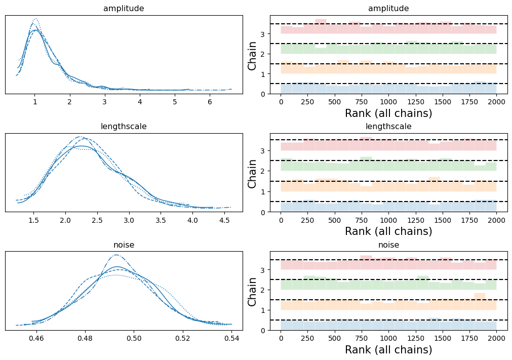
我们看到模型准确地恢复了生成核的超参数。(回想一下,核 amplitude 的值设置为 1.0,lengthscale 设置为 2.0)
[12]:
if INFERENCE == "mcmc":
    idata = az.from_numpyro(posterior=mcmc)
    mcmc.print_summary()
                   mean       std    median      5.0%     95.0%     n_eff     r_hat
    amplitude      1.31      0.57      1.17      0.58      2.11    868.30      1.00
  lengthscale      2.37      0.50      2.33      1.56      3.14    925.36      1.00
        noise      0.49      0.01      0.49      0.47      0.52   1307.16      1.00

Number of divergences: 0
检查单个链显示了收敛性。
[13]:
if INFERENCE == "mcmc":
    VAR_NAMES = ["amplitude", "lengthscale", "noise"]
    axes = az.plot_trace(
        data=idata,
        var_names=VAR_NAMES,
        kind="rank_bars",
        backend_kwargs={"figsize": (10, 7), "layout": "constrained"},
    )
现在,我们可以设置辅助函数,从后验预测中生成样本,并评估模型恢复已知函数形式和外推到边界的能力。
[14]:
def posterior_predictive_mcmc(
    seed: int,
    model: callable,
    mcmc: MCMC,
    **model_kwargs,
) -> dict[str, jax.Array]:
    samples = mcmc.get_samples()
    predictive = Predictive(model, samples, parallel=True)
    return predictive(random.PRNGKey(seed), **model_kwargs)


def posterior_predictive_svi(
    seed: int,
    model: callable,
    guide: callable,
    params: dict,
    num_samples: int = 2000,
    **model_kwargs,
) -> dict[str, jax.Array]:
    predictive = Predictive(model, guide=guide, params=params, num_samples=num_samples)
    return predictive(random.PRNGKey(seed), **model_kwargs)
使用后验样本,我们可以预测函数在网格点集上的值,并测试其恢复真实函数的能力。
[15]:
if INFERENCE == "mcmc":
    post_y = posterior_predictive_mcmc(seed, m.model, mcmc, X_test=X_grid)
else:
    post_y = posterior_predictive_svi(
        seed, m.model, guide, svi_res.params, X_test=X_grid
    )
通过从模型中抽取的后验预测样本,我们可以可视化潜在函数的样本以及相关的 80% 可信区间。
[16]:
def plot_fit_result(
    N_post: int, post: dict[str, jax.Array], q_lower: float = 0.1, q_upper: float = 0.9
):
    ci = np.quantile(post["y_test"], jnp.array([q_lower, q_upper]), axis=0)
    if D == 1:
        ci_lower, ci_upper = ci[0, :], ci[1, :]
        test_ind = (X < -L * tr_frac) | (X > L * tr_frac)
        ax = plot_line_scatter(
            X_grid,
            y_grid,
            X,
            y,
            test_ind=test_ind,
            post_y=post["f_star"][0:N_post, :],
            post_alpha=0.1,
            point_alpha=0.15,
            v_lines=[-L * tr_frac, L * tr_frac],
            ci=(ci_lower, ci_upper),
            fig_size=5.0,
        )
    elif D == 2:
        # compute confidence intervals at the edges of the grid
        yz_ind1 = X_grid[:, 0] == L
        yz_lower1 = ci[0, :][yz_ind1]
        yz_upper1 = ci[1, :][yz_ind1]
        yz_ind2 = X_grid[:, 0] == -L
        yz_lower2 = ci[0, :][yz_ind2]
        yz_upper2 = ci[1, :][yz_ind2]

        xz_ind1 = X_grid[:, 1] == L
        xz_lower1 = ci[0, :][xz_ind1]
        xz_upper1 = ci[1, :][xz_ind1]
        xz_ind2 = X_grid[:, 1] == -L
        xz_lower2 = ci[0, :][xz_ind2]
        xz_upper2 = ci[1, :][xz_ind2]

        ax = plot_surface_scatter(
            N_grid=N_grid,
            X_grid=X_grid,
            y_grid=y_grid,
            X=X,
            y=y,
            test_ind=~tr_idx,
            post_y=post["f_star"][0:N_post, :],
            post_alpha=0.1,
            xy_annotate_lines=[
                ((-L * tr_frac, -L * tr_frac), (-L * tr_frac, L * tr_frac)),
                ((-L * tr_frac, L * tr_frac), (L * tr_frac, L * tr_frac)),
                ((L * tr_frac, L * tr_frac), (-L * tr_frac, L * tr_frac)),
                ((L * tr_frac, -L * tr_frac), (-L * tr_frac, -L * tr_frac)),
            ],
            yz_lines=[
                (X_grid[yz_ind1, 1], yz_lower1, L),
                (X_grid[yz_ind1, 1], yz_upper1, L),
                (X_grid[yz_ind2, 1], yz_lower2, -L),
                (X_grid[yz_ind2, 1], yz_upper2, -L),
            ],
            xz_lines=[
                (X_grid[xz_ind1, 0], xz_lower1, L),
                (X_grid[xz_ind1, 0], xz_upper1, L),
                (X_grid[xz_ind2, 0], xz_lower2, -L),
                (X_grid[xz_ind2, 0], xz_upper2, -L),
            ],
            y_wireframe_alpha=0.4,
            ci_alpha=0.75,
        )
    return ax
[17]:
plot_fit_result(20, post_y)
plt.show()
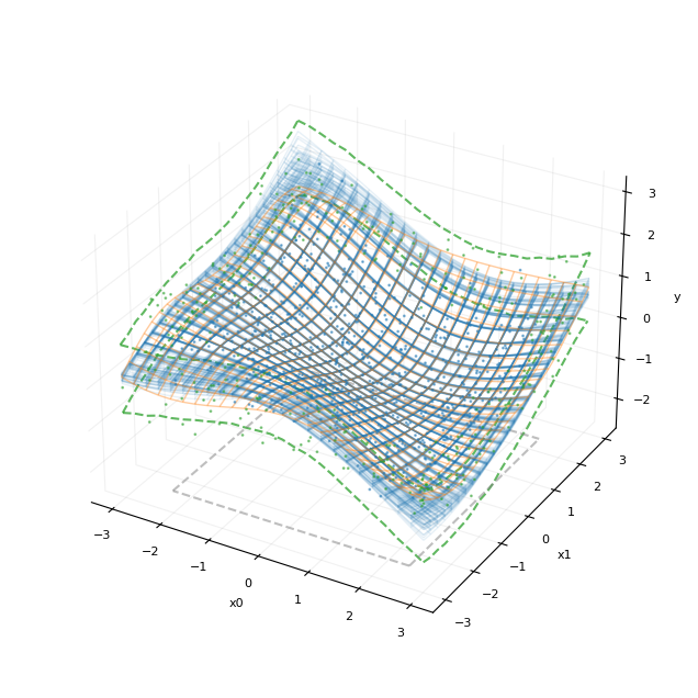
此处,我们将后验均值 (f_star) 的几个抽样绘制为蓝色线框图,叠加在橙色的真实函数上。x0-x1 平面中的正方形表示模型训练使用的数据区域。函数边界上的绿色虚线表示边界点处的 80% 可信区间。我们还绘制了蓝色的训练点集和绿色的测试点集。
我们还可以直接检查模型相对于网格点集的校准情况。plot_calibration 函数比较真实函数值与后验预测均值。
[18]:
def plot_calibration(
    y_true: jax.Array,
    y_pred: jax.Array,
    test_ind: jax.Array | None = None,
    fig_size: float = 5.0,
    label_size: float = 8.0,
    point_size: float = 1.0,
    x_label: str = "True",
    y_label: str = "Predicted",
):
    fig = plt.figure(figsize=(fig_size, fig_size))
    ax = fig.add_subplot()
    color = (
        "tab:blue" if test_ind is None else np.where(test_ind, "tab:green", "tab:blue")
    )
    ax.scatter(y_true, y_pred, c=color, alpha=0.5, s=point_size)
    ax.plot(
        [y_true.min(), y_true.max()],
        [y_true.min(), y_true.max()],
        color="tab:orange",
        linestyle="--",
    )
    ax.set_xlim([y_true.min(), y_true.max()])
    ax.set_ylim([y_true.min(), y_true.max()])
    ax.xaxis.set_tick_params(labelsize=label_size)
    ax.set_xlabel(x_label, fontsize=label_size)
    ax.yaxis.set_tick_params(labelsize=label_size)
    ax.set_ylabel(y_label, fontsize=label_size)
    return ax
[19]:
ax = plot_calibration(
    y_grid,
    post_y["f_star"].mean(axis=0),
    test_ind=~tr_idx_grid,
    point_size=1.0 if D == 2 else 5.0,
)
plt.show()
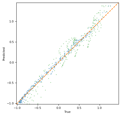
测试集范围内包含的网格点显示为蓝色。训练边界外的点显示为绿色。橙色的虚线是恒等线(真实值=预测值)。
最后,作为与 HSGP 近似进行比较的基准,我们计算(带噪声的)测试点集上的均方根误差。
[20]:
if INFERENCE == "mcmc":
    post_y_test = posterior_predictive_mcmc(seed, m.model, mcmc, X_test=X_test)
else:
    post_y_test = posterior_predictive_svi(
        seed, m.model, guide, svi_res.params, X_test=X_test
    )
print(
    "Test RMSE:",
    jnp.sqrt(jnp.mean((post_y_test["y_test"].mean(axis=0) - y_test) ** 2)),
)
Test RMSE: 0.5625003036885073
HSGP 替代方法
现在我们来看希尔伯特空间近似。Mayol 等人 2020 对该方法提供了易于理解且实用的介绍。Orduz 2024 另外提供了一个带有 numpyro 代码的详细一维示例教程。下面,我们演示了 numpyro.contrib.hsgp 模块在多维问题上的用法。完整的近似由下式给出:
(Mayol 等人 2020,式 14)
此处,\(S_{\theta}^\star\) 是平方指数核的光谱密度,\(\boldsymbol{\lambda}_j^\star\) 是拉普拉斯算子的特征值,\(\phi_j^\star\) 是拉普拉斯算子的特征函数,而 \(\beta_j\) 是展开式的系数(\(\sim \mathcal{N}(0, 1)\))。特征函数的总数是 \(m^\star\),它是每个维度的近似函数数量的乘积。
这个近似方便地由 numpyro.contrib.hsgp.approximation 模块的 hsgp_squared_exponential 函数实现。对于完整模型,我们只需采样核超参数,将这些超参数输入到 hsgp_squared_exponential 函数中,并定义发射分布。问题的维度从 X 的尾随维度推断。我们将每个维度的基函数数量(m)设置为 5,模型的支持区间([-L, L])设置为数据支持区间的 2.5 倍。如果需要,我们可以将长度为 D 的列表传递给 m 和 L,以允许近似的基函数数量和近似区间的长度因维度而异。
[21]:
@jax.tree_util.register_pytree_node_class
class HSGPModel:
    def __init__(self, m: int, L: float) -> None:
        self.m = m
        self.L = L

    def model(
        self,
        X: jax.Array,
        y: jax.Array | None = None,
    ):
        amplitude = numpyro.sample("amplitude", dist.LogNormal(0, 1))
        length = numpyro.sample("lengthscale", dist.Exponential(1))
        noise = numpyro.sample("noise", dist.LogNormal(0, 1))

        f = numpyro.deterministic(
            "f_star",
            hsgp_squared_exponential(
                X, alpha=amplitude, length=length, ell=self.L, m=self.m
            ),
        )
        site = "y" if y is not None else "y_test"
        numpyro.sample(site, dist.Normal(f, noise), obs=y)

    def tree_flatten(self):
        children = ()  # arrays / dynamic values
        aux_data = (
            self.L,
            self.m,
        )  # static values
        return (children, aux_data)

    @classmethod
    def tree_unflatten(cls, aux_data, children):
        return cls(*children, **aux_data)
我们可以使用上面相同的辅助函数来拟合模型。
[22]:
hsgp_m = HSGPModel(m=5, L=L * 2.5)

if INFERENCE == "mcmc":
    hsgp_mcmc = fit_mcmc(
        2,
        hsgp_m.model,
        X=X_tr,
        y=y_tr,
        num_warmup=500,
        num_samples=500,
        target_accept_prob=0.95,
        init_strategy=init_to_median(num_samples=25),
    )
else:
    hsgp_guide = AutoNormal(hsgp_m.model, init_loc_fn=init_to_median(num_samples=25))
    hsgp_res = fit_svi(seed, hsgp_m.model, hsgp_guide, X=X_tr, y=y_tr, num_steps=10_000)
我们看到推断出的核超参数与精确模型的超参数非常接近(尽管不完全相同)。
[23]:
if INFERENCE == "mcmc":
    idata_hsgp = az.from_numpyro(posterior=hsgp_mcmc)
    hsgp_mcmc.print_summary()
                   mean       std    median      5.0%     95.0%     n_eff     r_hat
    amplitude      1.90      1.14      1.59      0.59      3.43    926.95      1.00
      beta[0]      0.58      0.35      0.55      0.07      1.19   1259.52      1.00
      beta[1]     -1.48      0.46     -1.43     -2.18     -0.70   1487.24      1.00
      beta[2]      0.98      0.63      0.98      0.03      2.12   1209.91      1.00
      beta[3]     -1.03      0.49     -1.03     -1.82     -0.20   1723.47      1.00
      beta[4]     -0.14      0.68     -0.13     -1.27      0.91   1338.82      1.00
      beta[5]      1.20      0.51      1.15      0.44      2.11   1124.16      1.00
      beta[6]      0.06      0.57      0.05     -0.90      0.94   1697.33      1.00
      beta[7]     -0.72      0.77     -0.70     -1.90      0.62   1567.92      1.00
      beta[8]     -0.85      0.69     -0.84     -1.91      0.36   2049.00      1.00
      beta[9]     -0.48      0.81     -0.48     -1.89      0.82   1857.53      1.00
     beta[10]      0.31      0.63      0.31     -0.74      1.32   1457.68      1.00
     beta[11]     -0.82      0.87     -0.82     -2.23      0.60   1293.00      1.00
     beta[12]     -0.92      0.80     -0.91     -2.19      0.41   1939.01      1.00
     beta[13]      0.90      0.83      0.90     -0.46      2.27   1853.92      1.00
     beta[14]      0.13      0.85      0.10     -1.35      1.46   2544.06      1.00
     beta[15]     -0.11      0.50     -0.10     -0.90      0.75   1396.14      1.00
     beta[16]      0.93      0.69      0.92     -0.23      2.01   2263.74      1.00
     beta[17]      0.18      0.84      0.18     -1.25      1.47   1521.81      1.00
     beta[18]     -0.09      0.77     -0.09     -1.35      1.17   2366.62      1.00
     beta[19]      0.49      0.85      0.52     -0.88      1.87   1997.09      1.00
     beta[20]      0.07      0.68      0.07     -1.09      1.10   1524.95      1.00
     beta[21]      1.05      0.80      1.05     -0.26      2.39   2228.70      1.00
     beta[22]      0.26      0.90      0.28     -1.15      1.76   2297.64      1.00
     beta[23]     -0.21      0.85     -0.22     -1.60      1.17   2378.74      1.00
     beta[24]     -0.07      0.84     -0.06     -1.50      1.26   2027.63      1.00
  lengthscale      2.14      0.55      2.17      1.17      3.00    615.67      1.00
        noise      0.50      0.01      0.49      0.47      0.52   2482.71      1.00

Number of divergences: 0
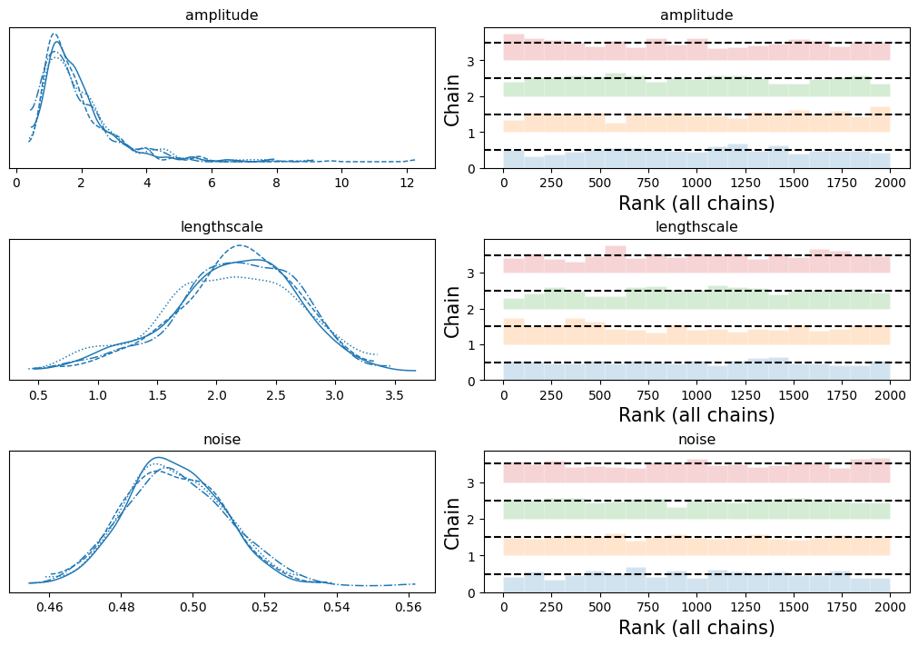
链条混合良好,与精确模型一样。
[24]:
if INFERENCE == "mcmc":
    axes = az.plot_trace(
        data=idata_hsgp,
        var_names=VAR_NAMES,
        kind="rank_bars",
        backend_kwargs={"figsize": (10, 7), "layout": "constrained"},
    )
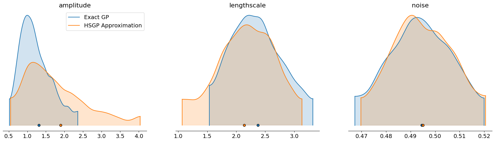
我们还可以使用 arviz 的 plot_density 函数,叠加精确模型和近似模型中核超参数的后验样本。
[25]:
axes = az.plot_density(
    [idata, idata_hsgp],
    data_labels=["Exact GP", "HSGP Approximation"],
    var_names=VAR_NAMES,
    shade=0.2,
)
我们可以像上面一样为网格点生成预测。
[26]:
if INFERENCE == "mcmc":
    post_y_hsgp = posterior_predictive_mcmc(seed, hsgp_m.model, hsgp_mcmc, X=X_grid)
else:
    post_y_hsgp = posterior_predictive_svi(
        seed,
        hsgp_m.model,
        hsgp_guide,
        hsgp_res.params,
        X=X_grid,
    )
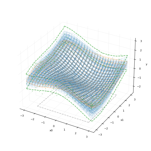
与精确模型一样,该近似能够准确地恢复函数的形状并很好地外推到边界。
[27]:
plot_fit_result(20, post_y_hsgp)
plt.show()
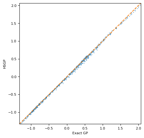
现在我们可以将近似模型的后验预测均值与精确模型的预测结果进行比较。我们看到近似模型与精确模型非常匹配。
[28]:
ax = plot_calibration(
    post_y["f_star"].mean(axis=0),
    post_y_hsgp["f_star"].mean(axis=0),
    point_size=1.0 if D == 2 else 5.0,
    x_label="Exact GP",
    y_label="HSGP",
)
plt.show()
近似模型在测试集上表现良好。
[29]:
if INFERENCE == "mcmc":
    post_y_test_hsgp = posterior_predictive_mcmc(
        seed, hsgp_m.model, hsgp_mcmc, X=X_test
    )
else:
    post_y_test_hsgp = posterior_predictive_svi(
        seed, hsgp_m.model, hsgp_guide, hsgp_res.params, X=X_test
    )
print(
    "Test RMSE:",
    jnp.sqrt(jnp.mean((post_y_test_hsgp["y_test"].mean(axis=0) - y_test) ** 2)),
)
Test RMSE: 0.5647539777438082