注意
到末尾下载完整的示例代码。
示例:VAR(2) 过程
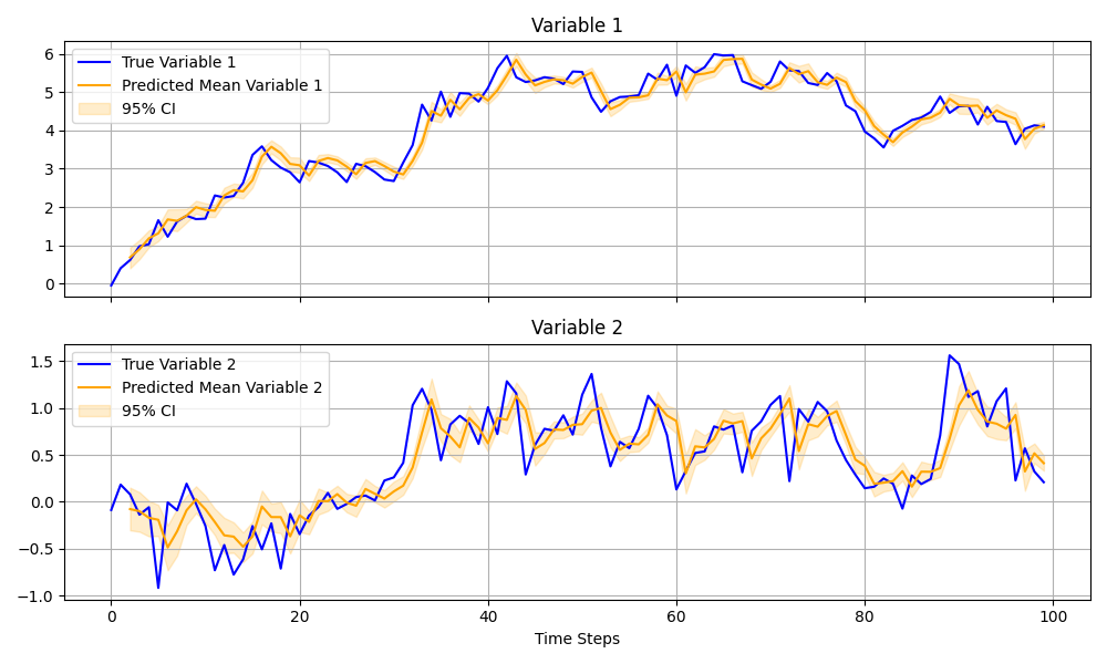
在本示例中,我们将演示如何实现向量自回归二阶过程 (VAR(2)) 并对其进行贝叶斯推断。VAR 模型在时间序列分析中被广泛应用,尤其适用于捕捉多个变量之间的动态关系。
对于包含 \(K\) 个变量的多元时间序列 \(y_t\),VAR(2) 过程定义为
\[y_t = c + \Phi_1 y_{t-1} + \Phi_2 y_{t-2} + \epsilon_t\]
这里,\(c\) 是一个常数向量,\(\Phi_1\) 和 \(\Phi_2\) 分别是滞后 1 和滞后 2 的系数矩阵,\(\epsilon_t\) 是一个零均值、协方差矩阵为 \(\Sigma\) 的高斯噪声项。
本示例使用 NumPyro 的 scan 工具来有效建模时间依赖性,避免显式的 Python 循环。
有关更通用的时间序列预测技术和示例,请参阅时间序列预测教程:https://num.pyro.org.cn/en/stable/tutorials/time_series_forecasting.html#Forecasting
参考
有关向量自回归模型的更多信息,请参阅:https://otexts.com/fpp2/VAR.html
import argparse
import os
import time

import matplotlib.pyplot as plt
import numpy as np

from jax import random
import jax.numpy as jnp

import numpyro
from numpyro.contrib.control_flow import scan
import numpyro.distributions as dist


def var2_scan(y):
    T, K = y.shape  # Number of time steps and number of variables

    # Priors for constants and coefficients
    c = numpyro.sample("c", dist.Normal(0, 1).expand([K]))  # Constants vector of size K
    Phi1 = numpyro.sample(
        "Phi1", dist.Normal(0, 1).expand([K, K]).to_event(2)
    )  # Coefficients for lag 1
    Phi2 = numpyro.sample(
        "Phi2", dist.Normal(0, 1).expand([K, K]).to_event(2)
    )  # Coefficients for lag 2

    # Priors for error terms
    sigma = numpyro.sample("sigma", dist.HalfNormal(1.0).expand([K]).to_event(1))
    L_omega = numpyro.sample(
        "L_omega", dist.LKJCholesky(dimension=K, concentration=1.0)
    )
    L_Sigma = (
        sigma[..., None] * L_omega
    )  # Alternative: jnp.einsum("...i,...ij->...ij", sigma, L_omega)

    def transition(carry, t):
        y_prev1, y_prev2, y_obs = carry  # Previous two observations and observed data
        m_t = c + jnp.dot(Phi1, y_prev1) + jnp.dot(Phi2, y_prev2)  # Mean prediction
        # Conditioned on observed y
        y_t = numpyro.sample(
            f"y_{t}",
            dist.MultivariateNormal(loc=m_t, scale_tril=L_Sigma),
            obs=y_obs[t],
        )
        new_carry = (y_t, y_prev1, y_obs)
        return new_carry, m_t

    # Initial carry: observations at time steps 1 and 0
    init_carry = (y[1], y[0], y[2:])

    # Time indices starting from time step 2
    time_indices = jnp.arange(T - 2)

    # Run the scan
    _, mu = scan(transition, init_carry, time_indices)

    # Store the mean trajectory as a deterministic variable
    numpyro.deterministic("mu", mu)


def generate_var2_data(T, K, c, Phi1, Phi2, sigma):
    """
    Generate time series data from a VAR(2) process.
    Args:
        T (int): Number of time steps.
        K (int): Number of variables in the time series.
        c (array): Constants (shape: (K,)).
        Phi1 (array): Coefficients for lag 1 (shape: (K, K)).
        Phi2 (array): Coefficients for lag 2 (shape: (K, K)).
        sigma (array): Covariance matrix for the noise (shape: (K, K)).
    Returns:
        np.ndarray: Generated time series data (shape: (T, K)).
    """
    # Initialize time series with random values
    y = np.zeros((T, K))
    y[:2] = np.random.multivariate_normal(mean=np.zeros(K), cov=sigma, size=2)

    # Generate the time series
    for t in range(2, T):
        y[t] = (
            c
            + Phi1 @ y[t - 1]
            + Phi2 @ y[t - 2]
            + np.random.multivariate_normal(mean=np.zeros(K), cov=sigma)
        )

    return y


def run_inference(model, args, rng_key, y):
    """
    Run MCMC inference for the given model.
    Args:
        model: The probabilistic model to infer.
        args: Command-line arguments.
        rng_key: PRNG key for randomness.
        y: Observed time series data.
    """
    start = time.time()
    sampler = numpyro.infer.NUTS(model)
    mcmc = numpyro.infer.MCMC(
        sampler,
        num_warmup=args.num_warmup,
        num_samples=args.num_samples,
        num_chains=args.num_chains,
        progress_bar=False if "NUMPYRO_SPHINXBUILD" in os.environ else True,
    )
    mcmc.run(rng_key, y=y)
    mcmc.print_summary()
    print("\nMCMC elapsed time:", time.time() - start)
    return mcmc.get_samples()


def main(args):
    # Generate artificial dataset
    T = args.num_data  # Number of time steps
    K = 2  # Number of variables
    c_true = jnp.array([0.5, -0.3])  # Constants
    Phi1_true = jnp.array([[0.7, 0.1], [0.2, 0.5]])  # Coefficients for lag 1
    Phi2_true = jnp.array([[0.2, -0.1], [-0.1, 0.2]])  # Coefficients for lag 2
    sigma_true = jnp.array([[0.1, 0.02], [0.02, 0.1]])  # Covariance matrix

    rng_key = random.PRNGKey(0)
    y = generate_var2_data(T, K, c_true, Phi1_true, Phi2_true, sigma_true)

    # Perform inference
    samples = run_inference(var2_scan, args, rng_key, y)

    # Prediction
    mean_prediction = samples["mu"].mean(axis=0)
    lower_bound = jnp.percentile(samples["mu"], 2.5, axis=0)  # 2.5th percentile
    upper_bound = jnp.percentile(samples["mu"], 97.5, axis=0)  # 97.5th percentile

    # Plot results
    fig, axes = plt.subplots(K, 1, figsize=(10, 6), sharex=True)
    time_steps = jnp.arange(T)

    for i in range(K):
        # True values
        axes[i].plot(time_steps, y[:, i], label=f"True Variable {i + 1}", color="blue")
        # Posterior mean prediction
        axes[i].plot(
            time_steps[2:],
            mean_prediction[:, i],
            label=f"Predicted Mean Variable {i + 1}",
            color="orange",
        )
        # 95% confidence interval
        axes[i].fill_between(
            time_steps[2:],
            lower_bound[:, i],
            upper_bound[:, i],
            color="orange",
            alpha=0.2,
            label="95% CI",
        )
        axes[i].set_title(f"Variable {i + 1}")
        axes[i].legend()
        axes[i].grid(True)

    plt.xlabel("Time Steps")
    plt.tight_layout()
    plt.savefig("var2.png")


if __name__ == "__main__":
    assert numpyro.__version__.startswith("0.18.0")
    parser = argparse.ArgumentParser(description="VAR(2) example")
    parser.add_argument("--num-data", nargs="?", default=100, type=int)
    parser.add_argument("-n", "--num-samples", nargs="?", default=1000, type=int)
    parser.add_argument("--num-warmup", nargs="?", default=1000, type=int)
    parser.add_argument("--num-chains", nargs="?", default=1, type=int)
    parser.add_argument("--device", default="cpu", type=str, help='use "cpu" or "gpu".')
    args = parser.parse_args()

    numpyro.set_platform(args.device)
    numpyro.set_host_device_count(args.num_chains)

    main(args)