时间序列预测
在本教程中,我们将演示如何在 NumPyro 中构建时间序列预测模型。具体来说,我们将复制 Rlgt: 具有趋势修改的贝叶斯指数平滑模型 包中的 季节性、全局趋势 (SGT) 模型。本教程将使用的时间序列数据是 lynx 数据集,其中包含 1821 年至 1934 年加拿大每年捕获的猞猁数量。
[ ]:
!pip install -q numpyro@git+https://github.com/pyro-ppl/numpyro
[1]:
import os

from IPython.display import set_matplotlib_formats
import matplotlib.pyplot as plt
import pandas as pd

from jax import random
import jax.numpy as jnp

import numpyro
from numpyro.contrib.control_flow import scan
from numpyro.diagnostics import autocorrelation, hpdi
import numpyro.distributions as dist
from numpyro.infer import MCMC, NUTS, Predictive

if "NUMPYRO_SPHINXBUILD" in os.environ:
    set_matplotlib_formats("svg")

numpyro.set_host_device_count(4)
assert numpyro.__version__.startswith("0.18.0")
数据
首先,让我们导入并查看数据集。
[2]:
URL = "https://raw.githubusercontent.com/vincentarelbundock/Rdatasets/master/csv/datasets/lynx.csv"
lynx = pd.read_csv(URL, index_col=0)
data = lynx["value"].values
print("Length of time series:", data.shape[0])
plt.figure(figsize=(8, 4))
plt.plot(lynx["time"], data)
plt.show()
Length of time series: 114
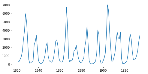
该时间序列的长度为 114(每年一个数据点),通过查看图表,我们可以观察到数据集中的季节性,即特定时间段内相似模式的周期性出现。例如,在该数据集中,我们观察到每 10 年出现一次周期性模式,但每 40 年捕获数量也会出现一个不太明显但清晰的峰值。让我们看看是否能在 NumPyro 中模拟这种效应。
在本教程中,我们将使用前 80 个值进行训练,使用后 34 个值进行测试。
[3]:
y_train, y_test = jnp.array(data[:80], dtype=jnp.float32), data[80:]
模型
我们将使用的模型称为 季节性、全局趋势 模型,该模型在针对 M-3 竞赛 中的 3003 个时间序列进行测试时,已知其性能优于最初参与竞赛的其他模型
\begin{align} \text{预期值}_{t} &= \text{基准值}_{t-1} + \text{趋势系数} \times \text{基准值}_{t-1}^{\text{趋势幂次}} + \text{季节分量}_t \times \text{基准值}_{t-1}^{\text{季节幂次}}, \\ \sigma_{t} &= \sigma \times \text{预期值}_{t}^{\text{幂次 x}} + \text{偏移量}, \\ y_{t} &\sim \text{学生 T 分布}(\nu, \text{预期值}_{t}, \sigma_{t}) \end{align}
,其中 level 和 s 遵循以下递归规则
\begin{align} \text{level-p} &= \begin{cases} y_t - \text{s}_t \times \text{level}_{t-1}^{\text{pow-season}} & \text{if } t \le \text{seasonality}, \\ \text{Average} \left[y(t - \text{seasonality} + 1), \ldots, y(t)\right] & \text{otherwise}, \end{cases} \\ \text{level}_{t} &= \text{level-sm} \times \text{level-p} + (1 - \text{level-sm}) \times \text{level}_{t-1}, \\ \text{s}_{t + \text{seasonality}} &= \text{s-sm} \times \frac{y_{t} - \text{level}_{t}}{\text{level}_{t-1}^{\text{pow-trend}}} + (1 - \text{s-sm}) \times \text{s}_{t}. \end{align}
有关 SGT 模型的更详细解释可在 Rlgt 包作者的此小插曲中找到。此处我们总结该模型的核心思想
学生 t 分布,其尾部比正态分布更厚重,用于似然函数。
期望值
exp_val由一个趋势分量和一个季节性分量组成趋势由映射 \(x \mapsto x + ax^b\) 控制,其中 \(x\) 是
level,\(a\) 是coef_trend,\(b\) 是pow_trend。请注意,当 \(b \sim 0\) 时,趋势是线性的,\(a\) 是斜率;当 \(b \sim 1\) 时,趋势是指数的,\(a\) 是增长率。因此,该函数可以覆盖广泛的趋势类别。当时间变化时,
level和s会更新到新值。系数level_sm和s_sm用于使过渡平滑。
当
powx接近 \(0\) 时,误差 \(\sigma_t\) 将几乎恒定,而当powx接近 \(1\) 时,误差将与期望值成比例。SGT 有多种变体。在本教程中,我们使用广义季节性和季节平均方法。
我们现在准备使用 NumPyro 基本构件指定模型。在 NumPyro 中,我们使用基本构件 sample(name, prior) 声明一个具有相应 prior 的潜在随机变量。这些基本构件可以根据 NumPyro 推断算法在后端使用的效果处理器具有自定义解释。例如,我们可以使用 condition 处理器在特定值上进行条件化,或者使用 trace 处理器在执行跟踪中记录这些采样点的值。请注意,这些细节对于指定模型或运行推断并不重要,但好奇的读者可以阅读 Pyro 中关于效果处理器的教程。
[4]:
def sgt(y, seasonality, future=0):
    # heuristically, standard derivation of Cauchy prior depends on
    # the max value of data
    cauchy_sd = jnp.max(y) / 150

    # NB: priors' parameters are taken from
    # https://github.com/cbergmeir/Rlgt/blob/master/Rlgt/R/rlgtcontrol.R
    nu = numpyro.sample("nu", dist.Uniform(2, 20))
    powx = numpyro.sample("powx", dist.Uniform(0, 1))
    sigma = numpyro.sample("sigma", dist.HalfCauchy(cauchy_sd))
    offset_sigma = numpyro.sample(
        "offset_sigma", dist.TruncatedCauchy(low=1e-10, loc=1e-10, scale=cauchy_sd)
    )

    coef_trend = numpyro.sample("coef_trend", dist.Cauchy(0, cauchy_sd))
    pow_trend_beta = numpyro.sample("pow_trend_beta", dist.Beta(1, 1))
    # pow_trend takes values from -0.5 to 1
    pow_trend = 1.5 * pow_trend_beta - 0.5
    pow_season = numpyro.sample("pow_season", dist.Beta(1, 1))

    level_sm = numpyro.sample("level_sm", dist.Beta(1, 2))
    s_sm = numpyro.sample("s_sm", dist.Uniform(0, 1))
    init_s = numpyro.sample("init_s", dist.Cauchy(0, y[:seasonality] * 0.3))

    def transition_fn(carry, t):
        level, s, moving_sum = carry
        season = s[0] * level**pow_season
        exp_val = level + coef_trend * level**pow_trend + season
        exp_val = jnp.clip(exp_val, 0)
        # use expected vale when forecasting
        y_t = jnp.where(t >= N, exp_val, y[t])

        moving_sum = (
            moving_sum + y[t] - jnp.where(t >= seasonality, y[t - seasonality], 0.0)
        )
        level_p = jnp.where(t >= seasonality, moving_sum / seasonality, y_t - season)
        level = level_sm * level_p + (1 - level_sm) * level
        level = jnp.clip(level, 0)

        new_s = (s_sm * (y_t - level) / season + (1 - s_sm)) * s[0]
        # repeat s when forecasting
        new_s = jnp.where(t >= N, s[0], new_s)
        s = jnp.concatenate([s[1:], new_s[None]], axis=0)

        omega = sigma * exp_val**powx + offset_sigma
        y_ = numpyro.sample("y", dist.StudentT(nu, exp_val, omega))

        return (level, s, moving_sum), y_

    N = y.shape[0]
    level_init = y[0]
    s_init = jnp.concatenate([init_s[1:], init_s[:1]], axis=0)
    moving_sum = level_init
    with numpyro.handlers.condition(data={"y": y[1:]}):
        _, ys = scan(
            transition_fn, (level_init, s_init, moving_sum), jnp.arange(1, N + future)
        )
    if future > 0:
        numpyro.deterministic("y_forecast", ys[-future:])
请注意,level 和 s 会递归更新,同时我们在每个时间步收集期望值。NumPyro 在后端使用 JAX 对 NUTS 算法的许多关键部分进行 JIT 编译,包括 Verlet 积分器和树构建过程。然而,如果在模型中使用 Python 的 for 循环这样做会导致模型的编译时间很长,因此我们使用 scan——它是 lax.scan 的一个封装,支持 NumPyro 基本构件和处理器。有关使用此实用程序的详细解释可在NumPyro 文档中找到。此处我们使用它收集 y 值,而三元组 (level, s, moving_sum) 扮演着携带状态的角色。
另一点需要注意的是,我们没有在 transition_fn 中声明观测站点 y
numpyro.sample("y", dist.StudentT(nu, exp_val, omega), obs=y[t])
,而是使用了 condition 处理器。原因是我们也想将此模型用于预测。在预测中,y 的未来值是不可观测的,因此当 t >= len(y) 时,obs=y[t] 没有意义(注意:JAX 不会引发索引越界错误,例如 jnp.arange(3)[10] == 2)。使用 condition,当 scan 的长度大于条件化/观测站点的长度时,未观测的值将从该站点的分布中进行采样。
推断
首先,我们想为 seasonality 选择一个好的值。按照 Rlgt 中的演示,我们将设置 seasonality=38。事实上,通过查看训练数据的图表可以猜到这个值,其中二阶季节性效应的周期性约为 \(40\) 年。注意,\(38\) 也是自相关最高的滞后之一。
[5]:
print("Lag values sorted according to their autocorrelation values:\n")
print(jnp.argsort(autocorrelation(y_train))[::-1])
Lag values sorted according to their autocorrelation values:

[ 0 67 57 38 68  1 29 58 37 56 28 10 19 39 66 78 47 77  9 79 48 76 30 18
 20 11 46 59 69 27 55 36  2  8 40 49 17 21 75 12 65 45 31 26  7 54 35 41
 50  3 22 60 70 16 44 13  6 25 74 53 42 32 23 43 51  4 15 14 34 24  5 52
 73 64 33 71 72 61 63 62]
现在,让我们运行 \(4\) 条 MCMC 链(使用 No-U-Turn Sampler 算法),每条链进行 \(5000\) 次预热步和 \(5000\) 次采样步。返回的值将是 \(20000\) 个样本的集合。
[6]:
%%time
kernel = NUTS(sgt)
mcmc = MCMC(kernel, num_warmup=5000, num_samples=5000, num_chains=4)
mcmc.run(random.PRNGKey(0), y_train, seasonality=38)
mcmc.print_summary()
samples = mcmc.get_samples()
                      mean       std    median      5.0%     95.0%     n_eff     r_hat
      coef_trend     32.33    123.99     12.07    -91.43    157.37   1307.74      1.00
       init_s[0]     84.35    105.16     61.08    -59.71    232.37   4053.35      1.00
       init_s[1]    -21.48     72.05    -26.11   -130.13     94.34   1038.51      1.01
       init_s[2]     26.08     92.13     13.57   -114.83    156.16   1559.02      1.00
       init_s[3]    122.52    123.56    102.67    -59.39    305.43   4317.17      1.00
       init_s[4]    443.91    254.12    395.89     69.08    789.27   3090.34      1.00
       init_s[5]   1163.56    491.37   1079.23    481.92   1861.90   1562.40      1.00
       init_s[6]   1968.70    649.68   1860.04    902.00   2910.49   1974.42      1.00
       init_s[7]   3652.34   1107.27   3505.37   1967.67   5383.26   1669.91      1.00
       init_s[8]   2593.04    831.42   2452.27   1317.67   3858.55   1805.87      1.00
       init_s[9]    947.28    422.29    885.72    311.39   1589.56   3355.27      1.00
      init_s[10]     44.09    102.92     28.38   -105.25    203.73   1367.99      1.00
      init_s[11]     -2.25     52.92     -2.71    -86.51     72.90    611.35      1.01
      init_s[12]    -12.22     64.98    -13.67   -110.07     85.65    892.13      1.01
      init_s[13]     74.43    106.48     53.13    -79.73    225.92    658.08      1.01
      init_s[14]    332.98    255.28    281.72    -11.18    697.96   3685.55      1.00
      init_s[15]    965.80    389.00    893.29    373.98   1521.59   2575.80      1.00
      init_s[16]   1261.12    469.99   1191.83    557.98   1937.38   2300.48      1.00
      init_s[17]   1372.34    559.14   1274.21    483.96   2151.94   2007.79      1.00
      init_s[18]    611.20    313.13    546.56    167.97   1087.74   2854.06      1.00
      init_s[19]     17.81     87.79      8.93   -118.64    143.96   5689.95      1.00
      init_s[20]    -31.84     66.70    -25.15   -146.89     58.97   3083.09      1.00
      init_s[21]    -14.01     44.74     -5.80    -86.03     42.99   2118.09      1.00
      init_s[22]     -2.26     42.99     -2.39    -61.40     66.34   3022.51      1.00
      init_s[23]     43.53     90.60     29.14    -82.56    167.89   3230.17      1.00
      init_s[24]    509.69    326.73    453.22     44.04    975.15   2087.02      1.00
      init_s[25]    919.23    431.15    837.03    284.54   1563.05   3257.27      1.00
      init_s[26]   1783.39    697.15   1660.09    720.83   2811.83   1730.70      1.00
      init_s[27]   1247.60    461.26   1172.88    544.44   1922.68   1573.09      1.00
      init_s[28]    217.92    169.08    191.38    -29.78    456.65   4899.06      1.00
      init_s[29]     -7.43     82.23    -12.99   -133.20    118.31   7588.25      1.00
      init_s[30]     -6.69     86.99    -17.03   -130.99    125.43   1687.37      1.00
      init_s[31]    -35.24     71.31    -35.75   -148.09     76.96   5462.22      1.00
      init_s[32]     -8.63     80.39    -14.95   -138.34    113.89   6626.25      1.00
      init_s[33]    117.38    148.71     91.69    -78.12    316.69   2424.57      1.00
      init_s[34]    502.79    297.08    448.55     87.88    909.45   1863.99      1.00
      init_s[35]   1064.57    445.88    984.10    391.61   1710.35   2584.45      1.00
      init_s[36]   1849.48    632.44   1763.31    861.63   2800.25   1866.47      1.00
      init_s[37]   1452.62    546.57   1382.62    635.28   2257.04   2343.09      1.00
        level_sm      0.00      0.00      0.00      0.00      0.00   7829.05      1.00
              nu     12.17      4.73     12.31      5.49     19.99   4979.84      1.00
    offset_sigma     31.82     31.84     22.43      0.01     73.13   1442.32      1.00
      pow_season      0.09      0.04      0.09      0.01      0.15   1091.99      1.00
  pow_trend_beta      0.26      0.18      0.24      0.00      0.52    199.20      1.01
            powx      0.62      0.13      0.62      0.40      0.84   2476.16      1.00
            s_sm      0.08      0.09      0.05      0.00      0.18   5866.57      1.00
           sigma      9.67      9.87      6.61      0.35     20.60   2376.07      1.00

Number of divergences: 4568
CPU times: user 1min 17s, sys: 108 ms, total: 1min 18s
Wall time: 41.2 s
预测
给定从 mcmc 中得到的 samples,我们想对测试数据集 y_test 进行预测。NumPyro 提供了一个便捷的实用工具 Predictive 来获取预测分布。让我们看看如何使用它来获取预测值。
请注意,在上面定义的 sgt 模型中,有一个关键字 future 控制模型的执行 - 取决于 future > 0 还是 future == 0。以下代码预测原始时间序列的最后 34 个值。
[7]:
predictive = Predictive(sgt, samples, return_sites=["y_forecast"])
forecast_marginal = predictive(random.PRNGKey(1), y_train, seasonality=38, future=34)[
    "y_forecast"
]
让我们计算 sMAPE、预测的均方根误差,并用平均预测和 90% 最高后验密度区间 (HPDI) 可视化结果。
[8]:
y_pred = jnp.mean(forecast_marginal, axis=0)
sMAPE = jnp.mean(jnp.abs(y_pred - y_test) / (y_pred + y_test)) * 200
msqrt = jnp.sqrt(jnp.mean((y_pred - y_test) ** 2))
print("sMAPE: {:.2f}, rmse: {:.2f}".format(sMAPE, msqrt))
sMAPE: 63.93, rmse: 1249.29
最后,让我们绘制结果图来验证我们是否得到了期望的结果。
[9]:
plt.figure(figsize=(8, 4))
plt.plot(lynx["time"], data)
t_future = lynx["time"][80:]
hpd_low, hpd_high = hpdi(forecast_marginal)
plt.plot(t_future, y_pred, lw=2)
plt.fill_between(t_future, hpd_low, hpd_high, alpha=0.3)
plt.title("Forecasting lynx dataset with SGT model (90% HPDI)")
plt.show()
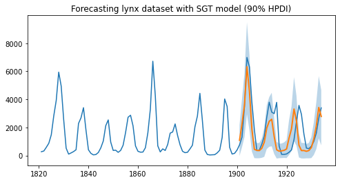
正如我们所观察到的,该模型能够学习一阶和二阶季节性效应,即周期性约为 10 的循环模式,以及大约每 40 年出现一次的峰值。此外,我们不仅有预测的点估计,还可以利用模型中的不确定性估计来限制我们的预测。
致谢
我们要感谢 Slawek Smyl 提供的许多有用的资源和建议。如果没有 JAX 和 XLA 团队的支持,快速推断是不可能实现的,因此我们要感谢他们为我们提供如此优秀的开源平台,以及他们对我们功能请求和 bug 报告的快速响应。
参考文献
[1] Rlgt: Bayesian Exponential Smoothing Models with Trend Modifications, Slawek Smyl, Christoph Bergmeir, Erwin Wibowo, To Wang Ng, Trustees of Columbia University