在线互动版本：

使用循环正态分布的快速高斯过程推断

高斯过程 (GP) 是用于函数数据建模的强大分布，但除了小数据集外，使用它们在计算上具有挑战性。快速傅里叶方法可以在数据位于规则网格上时有效评估似然。在本 notebook 中，我们使用 CirculantNormal 分布来推断带有二元观测的潜在 GP，并与标准 MultivariateNormal 进行比较。

总结：即使对于包含 64 个元素的的小型 GP，使用 CirculantNormal 也能在每秒有效样本数方面提供至少约 10 倍的加速。

我们考虑在规则网格 \(x\) 上的潜在高斯过程 \(z(x)\)，它编码了二元结果 \(y\) 的对数几率。更正式地，模型定义为

\[\begin{split}\begin{aligned} z&\sim\mathsf{MultivariateNormal}\left(0, K\right)\\ y&\sim\mathsf{Bernoulli}\left(\mathrm{expit} (z)\right), \end{aligned}\end{split}\]

其中 \(\mathrm{expit}(z) = 1/\left(1 + \exp(-z)\right)\) 表示逻辑 sigmoid，\(K\) 是在高斯过程元素之间在网格上评估得到的协方差矩阵。我们使用平方指数核 \(k\)，使得

\[\begin{split}\begin{aligned} K_{ij}&=k\left(x_i,x_j\right) + \epsilon \delta_{ij}\\ &=\sigma^2\exp\left(-\frac{d\left(x_i, x_j\right)}{2\ell^2}\right) \epsilon \delta_{ij}, \end{aligned}\end{split}\]

其中 \(\sigma\) 是高斯过程的边缘尺度，\(d\left(x_i, x_j\right)\) 是 \(x_i\) 和 \(x_j\) 之间的距离，而 \(\ell\) 是核的关联长度。我们在协方差矩阵的对角线上添加了一个所谓的“块金方差” \(\epsilon={10}^{-4}\)，以确保其数值正定。

CirculantNormal 分布需要循环协方差，即具有周期性边界条件的协方差。并非所有核都能表示，但可以通过填充域来减轻边界效应。

!pip install -q numpyro@git+https://github.com/pyro-ppl/numpyro matplotlib

生成合成数据

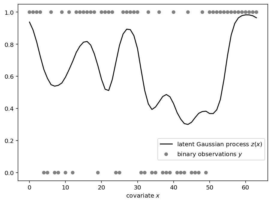
在此示例中，我们考虑 \(n=64\) 个等间距观测值，关联长度 \(\ell=5\) 和边缘尺度 \(\sigma=2\)。根据下面模型中的 method 参数，使用 CirculantNormal 或 MultivariateNormal 对 \(z\) 进行采样。

from time import time

from matplotlib import pyplot as plt

import jax
from jax import numpy as jnp, random
from jax.scipy.special import expit

import numpyro
from numpyro import distributions as dist


def model(x: jnp.ndarray, y: jnp.ndarray = None, *, method: str):
    """
    Latent Gaussian process model with binary outcomes.

    Args:
        x: Observation grid.
        y: Binary outcomes.
        method: Likelihood evaluation method.
    """
    n = x.size

    # Sample parameters and evaluate the kernel.
    sigma = numpyro.sample("sigma", dist.HalfNormal())
    length_scale = numpyro.sample("length_scale", dist.InverseGamma(5, 25))
    eps = 1e-4

    if method == "circulant":
        # We can evaluate the rfft of the covariance matrix directly. This both saves us
        # some computation and is more numerically stable.
        nrfft = n // 2 + 1
        k = jnp.arange(nrfft)
        covariance_rfft = (
            sigma**2
            * length_scale
            * jnp.sqrt(2 * jnp.pi)
            * jnp.exp(-2 * (jnp.pi * k * length_scale / n) ** 2)
        ) + eps
        zdist = dist.CirculantNormal(jnp.zeros(n), covariance_rfft=covariance_rfft)
    elif method == "cholesky":
        # Evaluate the covariance matrix.
        distance = jnp.abs(x[:, None] - x)
        distance = jnp.minimum(distance, n - distance)
        covariance_matrix = sigma**2 * jnp.exp(
            -(distance**2) / (2 * length_scale**2)
        ) + eps * jnp.eye(n)
        zdist = dist.MultivariateNormal(covariance_matrix=covariance_matrix)
    z = numpyro.sample("z", zdist)

    with numpyro.plate("n", n):
        numpyro.sample("y", dist.BernoulliLogits(z), obs=y)

定义模型后，我们使用 substitute 处理器指定合成数据的参数，使用 seed 处理器初始化随机数密钥，使用 trace 处理器记录模型执行，并可视化合成数据。

# Sample from the prior predictive.
with (
    numpyro.handlers.trace() as trace,
    numpyro.handlers.substitute(data={"sigma": 2, "length_scale": 5}),
    numpyro.handlers.seed(rng_seed=9),
):
    x = jnp.arange(64)
    model(x, method="circulant")
y = trace["y"]["value"]


# Plot the synthetic data.
def plot_data(x, trace, ax):
    ax.plot(
        x, expit(trace["z"]["value"]), label="latent Gaussian process $z(x)$", color="k"
    )
    ax.scatter(
        x, y, label="binary observations $y$", alpha=0.5, edgecolor="none", color="k"
    )
    ax.set_xlabel("covariate $x$")


fig, ax = plt.subplots()
plot_data(x, trace, ax=ax)
ax.legend(loc="lower right", bbox_to_anchor=(1, 0.1))
fig.tight_layout()

从后验采样

我们使用无掉头采样器 (NUTS) 使用这两种方法从后验中抽取样本。我们还记录了每秒有效样本数，这是评估采样器性能的常用指标。

samples_by_method = {}
n_eff_per_second_by_method = {}
for method in ["circulant", "cholesky"]:
    # Sample from the posterior using the NUTS kernel and record the duration.
    kernel = numpyro.infer.NUTS(model)
    mcmc = numpyro.infer.MCMC(kernel, num_warmup=800, num_samples=200)
    start = time()
    mcmc.run(random.key(9), x, trace["y"]["value"], method=method)
    duration = time() - start

    # Calculate the number of effective samples per second.
    samples_by_method[method] = mcmc.get_samples()
    n_eff_per_second_by_method[method] = {
        name: site["n_eff"] / duration
        for name, site in numpyro.diagnostics.summary(
            mcmc.get_samples(group_by_chain=True)
        ).items()
    }
    print(f"completed sampling in {duration:.3f} seconds for {method} method")

sample: 100%|████████████████████████████████████████████████████████| 1000/1000 [00:08<00:00, 123.94it/s, 255 steps of size 5.30e-03. acc. prob=0.89]

completed sampling in 12.800 seconds for circulant method

sample: 100%|████████████████████████████████████████████████████████| 1000/1000 [04:46<00:00,  3.48it/s, 1023 steps of size 5.02e-03. acc. prob=0.85]

completed sampling in 288.168 seconds for cholesky method

抽取后验样本后，我们将其可视化并与我们用于拟合模型的合成数据进行比较。下图显示了后验中位数（线条）以及从第 5 到第 95 百分位数形成的带状区域。

fig, ax = plt.subplots()
plot_data(x, trace, ax=ax)
for method, samples in samples_by_method.items():
    lower, median, upper = jnp.percentile(
        expit(samples["z"]), jnp.array([5, 50.0, 95]), axis=0
    )
    (line,) = ax.plot(x, median, label=method)
    ax.fill_between(x, lower, upper, color=line.get_color(), alpha=0.2)

ax.legend(loc="upper center", bbox_to_anchor=(0.5, 1.2), ncol=2)
fig.tight_layout()

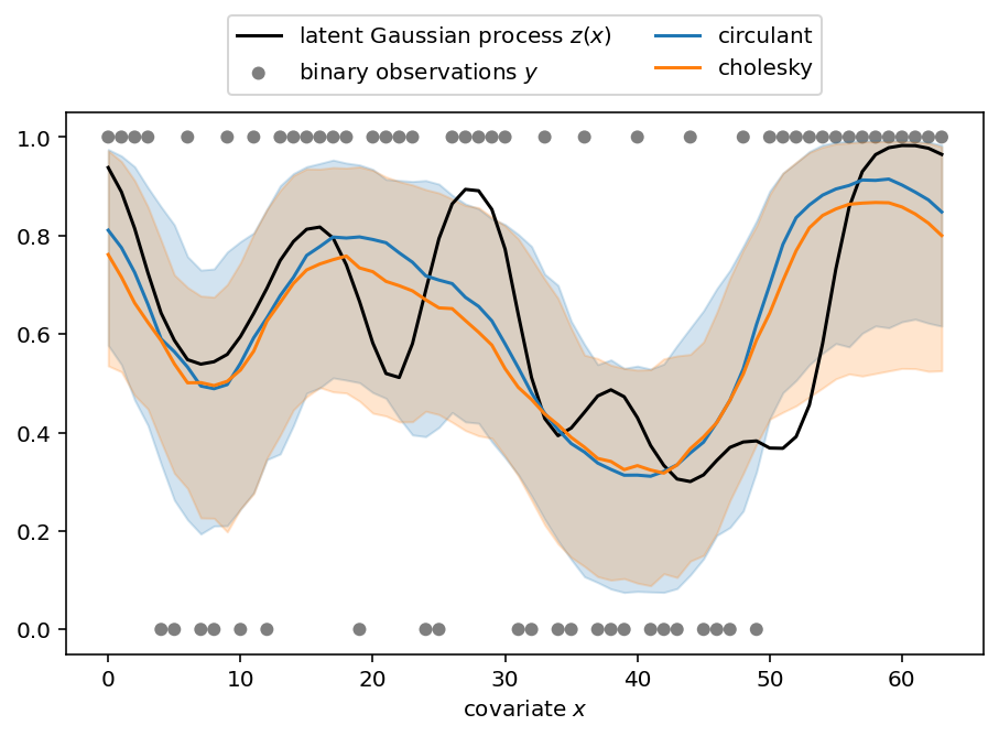
那么我们做得如何？使用 CirculantNormal 的运行时间快了约 20 倍。每秒有效样本数在不同参数之间有所差异，但根据参数不同，我们观察到 4 到 84 倍的改进。实验是在配备 M1 芯片的 2020 款 Macbook Pro 上进行的。

# Report the speed up due to using the `CirculantNormal`.
speedups = jax.tree.map(jnp.divide, *n_eff_per_second_by_method.values())
for site, speedup in speedups.items():
    print(
        f"speedup for `{site}`: min = {speedup.min():.2f}, "
        f"mean = {speedup.mean():.2f}, max = {speedup.max():.2f}"
    )

speedup for `length_scale`: min = 10.88, mean = 10.88, max = 10.88
speedup for `sigma`: min = 84.40, mean = 84.40, max = 84.40
speedup for `z`: min = 4.78, mean = 34.19, max = 80.74