使用 NumPyro 进行基于文本的理想点建模
Szymon Sacher & Keyon Vafa 本笔记本复现了基于文本的理想点模型 (Vafa, Naidu & Blei, 2020)
本笔记本设计用于在 Google Colab 上运行。
重要提示:为了保存此代码和您的结果,请确保将其复制到您的个人 Google 云端硬盘。在“文件”下,选择“在云端硬盘中保存副本”。
使用此 Colab 笔记本运行基于文本的理想点模型 (TBIP) TBIP 模型 的 NumPyro 实现,并处理政治文本语料库。 GitHub 仓库更完整。
另请参见此笔记本基于的 Tensorflow 实现。
TBIP 是一个无监督的概率主题模型,它通过分析文本来量化其作者的政治立场。该模型不使用政党或投票数据,也不需要任何按意识形态标记的文本。给定政治文本语料库和每篇文档的作者,TBIP 估计作者的潜在政治立场,以及每主题的词语选择如何随着作者的政治立场变化(“意识形态主题”)。请参阅论文了解更多信息。
入门
首先,确保您正在使用 GPU 运行此 Colab。转到“运行时”菜单,然后点击“更改运行时类型”。如果“硬件加速器”显示为“无”或“TPU”,请更改为“GPU”。点击“保存”即可开始。此外,如第一个单元格所述,请确保将此代码复制到您的个人 Google 云端硬盘。
安装 NumPyro
NumPyro 是一个概率编程框架,由 JAX 提供支持,用于 GPU/TPU/CPU 上的自动微分和即时编译。
[1]:
%%capture
%pip install numpyro==0.10.1
%pip install optax
克隆 TBIP 仓库
下面我们克隆 TBIP 的 GitHub 仓库。数据位于此处。
[2]:
! git clone https://github.com/keyonvafa/tbip
fatal: destination path 'tbip' already exists and is not an empty directory.
超参数和初始化
我们首先设置一些超参数。我们将主题数 \(K = 50\) 固定。我们还设置一个随机种子以确保结果的可复现性。
[3]:
from jax import random

num_topics = 50
rng_seed = random.PRNGKey(0)
下一个单元格提供了数据目录。下面单元格中的目录链接到 tbip 仓库中第 114 届参议院会议的演讲。
要使用您自己的语料库,请将以下四个文件上传到 Colab 工作目录:
counts.npz:一个[num_documents, num_words]稀疏 CSR 矩阵,包含每篇文档的词频。author_indices.npy:一个[num_documents]向量,其中每个条目是一个整数,属于集合{0, 1, ..., num_authors - 1},表示counts.npz中对应文档的作者。vocabulary.txt:一个[num_words]长度的文件,其中每行表示词汇表中的对应词。author_map.txt:一个[num_authors]长度的文件,其中每行表示语料库中某位作者的姓名。
请参阅 参议院演讲干净数据,了解参议院演讲这四个文件的示例。 我们的设置脚本 包含从未处理的参议院演讲数据创建这四个文件的示例代码。
重要提示:如果您使用自己的语料库,在将四个文件上传到 Colab 工作目录后,请将以下行更改为 data_dir = '.'。
[4]:
import numpy as np
from scipy import sparse

import jax
import jax.numpy as jnp

dataPath = "tbip/data/senate-speeches-114/clean/"

# Load data
author_indices = jax.device_put(
    jnp.load(dataPath + "author_indices.npy"), jax.devices("gpu")[0]
)

counts = sparse.load_npz(dataPath + "counts.npz")

with open(dataPath + "vocabulary.txt", "r") as f:
    vocabulary = f.readlines()

with open(dataPath + "author_map.txt", "r") as f:
    author_map = f.readlines()

author_map = np.array(author_map)

num_authors = int(author_indices.max() + 1)
num_documents, num_words = counts.shape
在论文中,参数使用 泊松分解 进行预初始化。大多数时候,我们发现这对于学习到的理想点没有太大区别,但有助于解释意识形态主题。
下面,我们使用 Scikit-Learn 的非负矩阵分解 (NMF) 实现进行初始化。尽管我们发现泊松分解学习到的主题更易于解释,但这里我们使用 Scikit-Learn 的 NMF 实现因为它更快。要使用泊松分解,请参阅 GitHub 仓库中的代码。
如果您想跳过此预初始化步骤,请在下面的单元格中设置 pre_initialize_parameters = False。(建议进行预初始化。)
[5]:
pre_initialize_parameters = True
如果正在进行参数预初始化,下面的单元格可能需要一分钟左右。
[6]:
# Fit NMF to be used as initialization for TBIP
from sklearn.decomposition import NMF

if pre_initialize_parameters:
    nmf_model = NMF(
        n_components=num_topics, init="random", random_state=0, max_iter=500
    )
    # Define initialization arrays
    initial_document_loc = jnp.log(
        jnp.array(np.float32(nmf_model.fit_transform(counts) + 1e-2))
    )
    initial_objective_topic_loc = jnp.log(
        jnp.array(np.float32(nmf_model.components_ + 1e-2))
    )
else:
    rng1, rng2 = random.split(rng_seed, 2)
    initial_document_loc = random.normal(rng1, shape=(num_documents, num_topics))
    initial_objective_topic_loc = random.normal(rng2, shape=(num_topics, num_words))
执行推断
我们使用 变分推断 和 重参数化 梯度 执行推断。下面提供简要总结,但鼓励读者 参阅原始论文 获得更完整的概述。
评估后验分布 \(p(\theta, \beta, \eta, x | y)\) 是难解的,因此我们使用参数化为 \(\phi\) 的分布 \(q_\phi(\theta, \beta,\eta,x)\) 来近似后验。我们如何设置 \(\phi\) 的值?我们希望最小化 \(q\) 与后验之间的 KL 散度,这等同于最大化 ELBO
我们将变分族设定为平均场族,这意味着潜在变量在文档 \(d\)、主题 \(k\) 和作者 \(s\) 上分解
我们对正值变量使用对数正态因子,对实值变量使用高斯因子
因此,我们的目标是最大化关于 \(\phi = \{\mu_\theta, \sigma_\theta, \mu_\beta, \sigma_\beta,\mu_\eta, \sigma_\eta, \mu_x, \sigma_x\}\) 的ELBO。
在下面的单元格中,我们定义模型和变分族(guide)。
[7]:
from numpyro import param, plate, sample
import numpyro.distributions as dist
from numpyro.distributions import constraints

# Define the model and variational family


class TBIP:
    def __init__(self, N, D, K, V, batch_size, init_mu_theta=None, init_mu_beta=None):
        self.N = N  # number of people
        self.D = D  # number of documents
        self.K = K  # number of topics
        self.V = V  # number of words in vocabulary
        self.batch_size = batch_size  # number of documents in a batch

        if init_mu_theta is None:
            init_mu_theta = jnp.zeros([D, K])
        else:
            self.init_mu_theta = init_mu_theta

        if init_mu_beta is None:
            init_mu_beta = jnp.zeros([K, V])
        else:
            self.init_mu_beta = init_mu_beta

    def model(self, Y_batch, d_batch, i_batch):
        with plate("i", self.N):
            # Sample the per-unit latent variables (ideal points)
            x = sample("x", dist.Normal())

        with plate("k", size=self.K, dim=-2):
            with plate("k_v", size=self.V, dim=-1):
                beta = sample("beta", dist.Gamma(0.3, 0.3))
                eta = sample("eta", dist.Normal())

        with plate("d", size=self.D, subsample_size=self.batch_size, dim=-2):
            with plate("d_k", size=self.K, dim=-1):
                # Sample document-level latent variables (topic intensities)
                theta = sample("theta", dist.Gamma(0.3, 0.3))

            # Compute Poisson rates for each word
            P = jnp.sum(
                jnp.expand_dims(theta, 2)
                * jnp.expand_dims(beta, 0)
                * jnp.exp(
                    jnp.expand_dims(x[i_batch], (1, 2)) * jnp.expand_dims(eta, 0)
                ),
                1,
            )

            with plate("v", size=self.V, dim=-1):
                # Sample observed words
                sample("Y_batch", dist.Poisson(P), obs=Y_batch)

    def guide(self, Y_batch, d_batch, i_batch):
        # This defines variational family. Notice that each of the latent variables
        # defined in the sample statements in the model above has a corresponding
        # sample statement in the guide. The guide is responsible for providing
        # variational parameters for each of these latent variables.

        # Also notice it is required that model and the guide have the same call.

        mu_x = param(
            "mu_x", init_value=-1 + 2 * random.uniform(random.PRNGKey(1), (self.N,))
        )
        sigma_x = param(
            "sigma_y", init_value=jnp.ones([self.N]), constraint=constraints.positive
        )

        mu_eta = param(
            "mu_eta", init_value=random.normal(random.PRNGKey(2), (self.K, self.V))
        )
        sigma_eta = param(
            "sigma_eta",
            init_value=jnp.ones([self.K, self.V]),
            constraint=constraints.positive,
        )

        mu_theta = param("mu_theta", init_value=self.init_mu_theta)
        sigma_theta = param(
            "sigma_theta",
            init_value=jnp.ones([self.D, self.K]),
            constraint=constraints.positive,
        )

        mu_beta = param("mu_beta", init_value=self.init_mu_beta)
        sigma_beta = param(
            "sigma_beta",
            init_value=jnp.ones([self.K, self.V]),
            constraint=constraints.positive,
        )

        with plate("i", self.N):
            sample("x", dist.Normal(mu_x, sigma_x))

        with plate("k", size=self.K, dim=-2):
            with plate("k_v", size=self.V, dim=-1):
                sample("beta", dist.LogNormal(mu_beta, sigma_beta))
                sample("eta", dist.Normal(mu_eta, sigma_eta))

        with plate("d", size=self.D, subsample_size=self.batch_size, dim=-2):
            with plate("d_k", size=self.K, dim=-1):
                sample("theta", dist.LogNormal(mu_theta[d_batch], sigma_theta[d_batch]))

    def get_batch(self, rng, Y, author_indices):
        # Helper functions to obtain a batch of data, convert from scipy.sparse
        # to jax.numpy.array and move to gpu

        D_batch = random.choice(rng, jnp.arange(self.D), shape=(self.batch_size,))
        Y_batch = jax.device_put(jnp.array(Y[D_batch].toarray()), jax.devices("gpu")[0])
        D_batch = jax.device_put(D_batch, jax.devices("gpu")[0])
        I_batch = author_indices[D_batch]
        return Y_batch, I_batch, D_batch
初始化
下面我们初始化一个TBIP模型实例及其关联的SVI对象。后者用于根据guide当前参数值和当前数据批次计算证据下界(ELBO)。
我们使用Adam优化器和指数衰减的学习率来优化模型。
[8]:
# Initialize the model
from jax import jit
from optax import adam, exponential_decay

from numpyro.infer import SVI, TraceMeanField_ELBO

num_steps = 50000
batch_size = 512  # Large batches are recommended
learning_rate = 0.01
decay_rate = 0.01

tbip = TBIP(
    N=num_authors,
    D=num_documents,
    K=num_topics,
    V=num_words,
    batch_size=batch_size,
    init_mu_theta=initial_document_loc,
    init_mu_beta=initial_objective_topic_loc,
)

svi_batch = SVI(
    model=tbip.model,
    guide=tbip.guide,
    optim=adam(exponential_decay(learning_rate, num_steps, decay_rate)),
    loss=TraceMeanField_ELBO(),
)

# Compile update function for faster training
svi_batch_update = jit(svi_batch.update)

# Get initial batch. This informs the dimension of arrays and ensures they are
# consistent with dimensions (N, D, K, V) defined above.
Y_batch, I_batch, D_batch = tbip.get_batch(random.PRNGKey(1), counts, author_indices)

# Initialize the parameters using initial batch
svi_state = svi_batch.init(
    random.PRNGKey(0), Y_batch=Y_batch, d_batch=D_batch, i_batch=I_batch
)
[9]:
# @title Run this cell to create helper function for printing topics


def get_topics(
    neutral_mean, negative_mean, positive_mean, vocabulary, print_to_terminal=True
):
    num_topics, num_words = neutral_mean.shape
    words_per_topic = 10
    top_neutral_words = np.argsort(-neutral_mean, axis=1)
    top_negative_words = np.argsort(-negative_mean, axis=1)
    top_positive_words = np.argsort(-positive_mean, axis=1)
    topic_strings = []
    for topic_idx in range(num_topics):
        neutral_start_string = "Neutral  {}:".format(topic_idx)
        neutral_row = [
            vocabulary[word] for word in top_neutral_words[topic_idx, :words_per_topic]
        ]
        neutral_row_string = ", ".join(neutral_row)
        neutral_string = " ".join([neutral_start_string, neutral_row_string])

        positive_start_string = "Positive {}:".format(topic_idx)
        positive_row = [
            vocabulary[word] for word in top_positive_words[topic_idx, :words_per_topic]
        ]
        positive_row_string = ", ".join(positive_row)
        positive_string = " ".join([positive_start_string, positive_row_string])

        negative_start_string = "Negative {}:".format(topic_idx)
        negative_row = [
            vocabulary[word] for word in top_negative_words[topic_idx, :words_per_topic]
        ]
        negative_row_string = ", ".join(negative_row)
        negative_string = " ".join([negative_start_string, negative_row_string])

        if print_to_terminal:
            topic_strings.append(negative_string)
            topic_strings.append(neutral_string)
            topic_strings.append(positive_string)
            topic_strings.append("==========")
        else:
            topic_strings.append(
                "  \n".join([negative_string, neutral_string, positive_string])
            )

    if print_to_terminal:
        all_topics = "{}\n".format(np.array(topic_strings))
    else:
        all_topics = np.array(topic_strings)
    return all_topics
执行训练
上面的代码创建了模型;下面我们实际运行训练。您可以调整训练步数(num_steps,在上方定义)以及打印ELBO的频率(print_steps,在下方定义)。
这里,我们运行训练循环。主题摘要和排序的理想点将每隔2500步打印一次。通常在我们的实验中,大约需要15,000步才能开始看到合理的结果,但这当然取决于语料库。这些合理结果应在半小时内达到。对于默认的参议院演讲语料库,完成30,000训练步(即默认的 num_steps)应少于2小时。
[10]:
# Run SVI
import pandas as pd
from tqdm import tqdm

print_steps = 100
print_intermediate_results = False

rngs = random.split(random.PRNGKey(2), num_steps)
losses = []
pbar = tqdm(range(num_steps))


for step in pbar:
    Y_batch, I_batch, D_batch = tbip.get_batch(rngs[step], counts, author_indices)
    svi_state, loss = svi_batch_update(
        svi_state, Y_batch=Y_batch, d_batch=D_batch, i_batch=I_batch
    )

    loss = loss / counts.shape[0]
    losses.append(loss)
    if step % print_steps == 0 or step == num_steps - 1:
        pbar.set_description(
            "Init loss: "
            + "{:10.4f}".format(jnp.array(losses[0]))
            + f"; Avg loss (last {print_steps} iter): "
            + "{:10.4f}".format(jnp.array(losses[-100:]).mean())
        )

    if (step + 1) % 2500 == 0 or step == num_steps - 1:
        # Save intermediate results
        estimated_params = svi_batch.get_params(svi_state)

        neutral_mean = (
            estimated_params["mu_beta"] + estimated_params["sigma_beta"] ** 2 / 2
        )

        positive_mean = (
            estimated_params["mu_beta"]
            + estimated_params["mu_eta"]
            + (estimated_params["sigma_beta"] ** 2 + estimated_params["sigma_eta"] ** 2)
            / 2
        )

        negative_mean = (
            estimated_params["mu_beta"]
            - estimated_params["mu_eta"]
            + (estimated_params["sigma_beta"] ** 2 + estimated_params["sigma_eta"] ** 2)
            / 2
        )

        np.save("neutral_topic_mean.npy", neutral_mean)
        np.save("negative_topic_mean.npy", positive_mean)
        np.save("positive_topic_mean.npy", negative_mean)

        topics = get_topics(neutral_mean, positive_mean, negative_mean, vocabulary)

        with open("topics.txt", "w") as f:
            print(topics, file=f)

        authors = pd.DataFrame(
            {"name": author_map, "ideal_point": np.array(estimated_params["mu_x"])}
        )
        authors.to_csv("authors.csv")

        if print_intermediate_results:
            print(f"Results after {step} steps.")
            print(topics)
            sorted_authors = "Authors sorted by their ideal points: " + ",".join(
                list(authors.sort_values("ideal_point")["name"])
            )
            print(sorted_authors.replace("\n", " "))
Init loss: 14323.9385; Avg loss (last 100 iter):   953.5815:   5%|▍         | 2499/50000 [03:47<1:11:33, 11.06it/s]/usr/local/lib/python3.7/dist-packages/jax/_src/numpy/lax_numpy.py:3327: UserWarning: 'kind' argument to argsort is ignored; only 'stable' sorts are supported.
  warnings.warn("'kind' argument to argsort is ignored; only 'stable' sorts "
Init loss: 14323.9385; Avg loss (last 100 iter):   634.0942: 100%|██████████| 50000/50000 [1:17:57<00:00, 10.69it/s]
[11]:
import matplotlib.pyplot as plt
import seaborn as sns

neutral_topic_mean = np.load("neutral_topic_mean.npy")
negative_topic_mean = np.load("negative_topic_mean.npy")
positive_topic_mean = np.load("positive_topic_mean.npy")
authors = pd.read_csv("authors.csv")
authors["name"] = authors["name"].str.replace("\n", "")
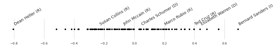
例如,这里是学习到的理想点的图。我们不标注每个点,因为点太多无法全部标注。下面我们选择一些作者进行标注。
[12]:
selected_authors = np.array(
    [
        "Dean Heller (R)",
        "Bernard Sanders (I)",
        "Elizabeth Warren (D)",
        "Charles Schumer (D)",
        "Susan Collins (R)",
        "Marco Rubio (R)",
        "John Mccain (R)",
        "Ted Cruz (R)",
    ]
)

sns.set(style="whitegrid")
fig = plt.figure(figsize=(12, 1))
ax = plt.axes([0, 0, 1, 1], frameon=False)
for index in range(authors.shape[0]):
    ax.scatter(authors["ideal_point"][index], 0, c="black", s=20)
    if authors["name"][index] in selected_authors:
        ax.annotate(
            author_map[index],
            xy=(authors["ideal_point"][index], 0.0),
            xytext=(authors["ideal_point"][index], 0),
            rotation=30,
            size=14,
        )
ax.set_yticks([])
plt.show()
自动生成guide
上面,出于教学目的,我们手动定义了guide(即变分族),确保它与原始论文中描述的完全相同。
然而,手动定义guide通常是不必要的,因为NumPyro包含一个可以根据提供的模型自动生成guide的模块。
在我们的例子中,结果表明 AutoNormal 创建的guide与我们在上面手动定义的guide完全相同。具体来说,它首先将变量变换到不受限制的实数空间。例如,对那些限制为非负的变量(文档位置 \(\theta_d\) 和客观主题位置 \(\beta_j\))应用对数变换。然后,它对每个变换后的分布使用独立的Normal分布作为guide。
在下面的单元格中,我们验证由 AutoNormal 生成的guide实际上与上面作为TBIP类一部分手动定义的guide完全相同。
[13]:
from numpyro.infer.autoguide import AutoNormal


def create_svi_object(guide):
    SVI(
        model=tbip.model,
        guide=guide,
        optim=adam(exponential_decay(learning_rate, num_steps, decay_rate)),
        loss=TraceMeanField_ELBO(),
    )

    Y_batch, I_batch, D_batch = tbip.get_batch(
        random.PRNGKey(1), counts, author_indices
    )

    svi_state = svi_batch.init(
        random.PRNGKey(0), Y_batch=Y_batch, d_batch=D_batch, i_batch=I_batch
    )

    return svi_state


# This state uses the guide defined manually above
svi_state_manualguide = create_svi_object(guide=tbip.guide)

# Now let's create this object but using AutoNormal guide. We just need to ensure that
# parameters are initialized as above.
autoguide = AutoNormal(
    model=tbip.model,
    init_loc_fn={"beta": initial_objective_topic_loc, "theta": initial_document_loc},
)
svi_state_autoguide = create_svi_object(guide=autoguide)


# Assert that the keys in the optimizer states are identical
assert svi_state_manualguide[0][1][0].keys() == svi_state_autoguide[0][1][0].keys()

# Assert that the values in the optimizer states are identical
for key in svi_state_manualguide[0][1][0].keys():
    assert jnp.all(
        svi_state_manualguide[0][1][0][key] == svi_state_autoguide[0][1][0][key]
    )