交互式在线版本：

贝叶斯分层线性回归

作者：Carlos Souza

更新者：Chris Stoafer

概率机器学习模型不仅可以对未来数据进行预测，还可以对不确定性建模。在个性化医疗等领域，数据量可能很大，但针对每个患者的数据量仍然相对较少。为了针对每个人定制预测，有必要为每个人建立一个模型——包含其固有的不确定性——并将这些模型分层耦合在一起，以便可以借鉴其他相似人群的信息[1]。

本教程的目的是演示如何使用 NumPyro 实现贝叶斯分层线性回归模型。为了引出本教程，我将使用 Kaggle 上托管的OSIC 肺纤维化进展竞赛数据。

1. 理解任务

肺纤维化是一种病因不明、无法治愈的疾病，由肺部瘢痕形成引起。本次竞赛要求我们预测患者肺功能下降的严重程度。肺功能通过肺活量计的输出进行评估，肺活量计测量用力肺活量 (FVC)，即呼出的空气量。

在医疗应用中，评估模型对其决策的置信度非常有用。因此，用于排名团队的指标旨在反映每次预测的准确性和确定性。它是拉普拉斯对数似然的修改版本（稍后会详细介绍）。

让我们看看数据，了解其内容

!pip install -q numpyro@git+https://github.com/pyro-ppl/numpyro arviz

import matplotlib.pyplot as plt
import numpy as np
import pandas as pd
import seaborn as sns

train = pd.read_csv(
    "https://gist.githubusercontent.com/ucals/"
    "2cf9d101992cb1b78c2cdd6e3bac6a4b/raw/"
    "43034c39052dcf97d4b894d2ec1bc3f90f3623d9/"
    "osic_pulmonary_fibrosis.csv"
)
train.head()

	患者	周	FVC	百分比	年龄	性别	吸烟状态
0	ID00007637202177411956430	-4	2315	58.253649	79	男性	前吸烟者
1	ID00007637202177411956430	5	2214	55.712129	79	男性	前吸烟者
2	ID00007637202177411956430	7	2061	51.862104	79	男性	前吸烟者
3	ID00007637202177411956430	9	2144	53.950679	79	男性	前吸烟者
4	ID00007637202177411956430	11	2069	52.063412	79	男性	前吸烟者

在数据集中，我们获得了一组患者的基线胸部 CT 扫描和相关的临床信息。患者在第 0 周进行图像采集，并在约 1-2 年内进行多次随访，期间测量其 FVC。在本教程中，我将只使用患者 ID、周数和 FVC 测量值，其余全部丢弃。仅使用这些列就使我们的团队获得了有竞争力的分数，这显示了贝叶斯分层线性回归模型的强大之处，特别是在衡量不确定性是问题的重要组成部分时。

由于这是真实的医疗数据，FVC 测量的时间点差异很大，如下面的 3 个示例患者所示

def chart_patient(patient_id, ax):
    data = train[train["Patient"] == patient_id]
    x = data["Weeks"]
    y = data["FVC"]
    ax.set_title(patient_id)
    sns.regplot(x=x, y=y, ax=ax, ci=None, line_kws={"color": "red"})


f, axes = plt.subplots(1, 3, figsize=(15, 5))
chart_patient("ID00007637202177411956430", axes[0])
chart_patient("ID00009637202177434476278", axes[1])
chart_patient("ID00010637202177584971671", axes[2])

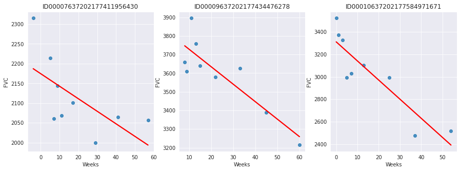
平均而言，提供的 176 名患者每人进行了 9 次随访，期间测量了 FVC。随访发生在 [-12, 133] 区间的特定周。肺活量下降非常明显。然而，我们看到不同患者之间差异很大。

我们被要求预测每个患者在 [-12, 133] 区间内所有可能周的 FVC 测量值，以及每次预测的置信度。换句话说：我们被要求填写一个如下所示的矩阵，并为每次预测提供置信度分数

这项任务非常适合应用贝叶斯推断。然而，Kaggle 社区分享的绝大多数解决方案使用了判别式机器学习模型，忽略了大多数判别式方法在提供现实不确定性估计方面的能力非常差的事实。因为它们通常以优化参数以最小化某个损失准则（例如，预测误差）的方式进行训练，所以它们通常不会在其参数或后续预测中编码任何不确定性。尽管许多方法可以通过副产品或后处理步骤产生不确定性估计，但这通常是基于启发式的，而不是自然地源于对目标不确定性分布的统计原理估计[2]。

2. 建模：具有部分汇集的贝叶斯分层线性回归

最简单的线性回归，非分层的，会假设所有 FVC 下降曲线具有相同的 \(\alpha\) 和 \(\beta\)。这就是完全汇集模型。在另一个极端，我们可以假设一个模型，其中每个患者都有个性化的 FVC 下降曲线，并且这些曲线完全无关。这就是不汇集模型，其中每个患者都有完全独立的回归。

这里，我将采用中间方案：部分汇集。具体来说，我将假设虽然 \(\alpha\) 和 \(\beta\) 对于每个患者来说是不同的，就像不汇集的情况一样，但这些系数都具有相似性。我们可以通过假设每个个体系数都来自一个共同的群体分布来对此建模。下图以图形方式表示此模型

在数学上，模型由以下方程描述

\begin{align} \mu_{\alpha} &\sim \text{正态分布}(0, 500) \\ \sigma_{\alpha} &\sim \text{半正态分布}(100) \\ \mu_{\beta} &\sim \text{正态分布}(0, 3) \\ \sigma_{\beta} &\sim \text{半正态分布}(3) \\ \alpha_i &\sim \text{正态分布}(\mu_{\alpha}, \sigma_{\alpha}) \\ \beta_i &\sim \text{正态分布}(\mu_{\beta}, \sigma_{\beta}) \\ \sigma &\sim \text{半正态分布}(100) \\ FVC_{ij} &\sim \text{正态分布}(\alpha_i + t \beta_i, \sigma) \end{align}

其中 t 是以周为单位的时间。这些先验信息量非常少，但这没关系：我们的模型会收敛的！

在 NumPyro 中实现这个模型非常简单

from jax import random

import numpyro
import numpyro.distributions as dist
from numpyro.infer import MCMC, NUTS, Predictive

assert numpyro.__version__.startswith("0.18.0")

def model(patient_code, Weeks, FVC_obs=None):
    μ_α = numpyro.sample("μ_α", dist.Normal(0.0, 500.0))
    σ_α = numpyro.sample("σ_α", dist.HalfNormal(100.0))
    μ_β = numpyro.sample("μ_β", dist.Normal(0.0, 3.0))
    σ_β = numpyro.sample("σ_β", dist.HalfNormal(3.0))

    n_patients = len(np.unique(patient_code))

    with numpyro.plate("plate_i", n_patients):
        α = numpyro.sample("α", dist.Normal(μ_α, σ_α))
        β = numpyro.sample("β", dist.Normal(μ_β, σ_β))

    σ = numpyro.sample("σ", dist.HalfNormal(100.0))
    FVC_est = α[patient_code] + β[patient_code] * Weeks

    with numpyro.plate("data", len(patient_code)):
        numpyro.sample("obs", dist.Normal(FVC_est, σ), obs=FVC_obs)

建模部分到此为止！

3. 拟合模型

NumPyro 等概率编程语言的一个伟大成就是将模型规范和推断解耦。在指定了包含先验、条件语句和数据似然的生成模型后，我可以将繁重的工作留给 NumPyro 的推断引擎。

调用它只需要几行代码。在此之前，让我们为每个患者代码添加一个数字患者 ID。这可以使用 scikit-learn 的 LabelEncoder 轻松完成

from sklearn.preprocessing import LabelEncoder

patient_encoder = LabelEncoder()
train["patient_code"] = patient_encoder.fit_transform(train["Patient"].values)

FVC_obs = train["FVC"].values
Weeks = train["Weeks"].values
patient_code = train["patient_code"].values

现在，调用 NumPyro 的推断引擎

nuts_kernel = NUTS(model)

mcmc = MCMC(nuts_kernel, num_samples=2000, num_warmup=2000)
rng_key = random.PRNGKey(0)
mcmc.run(rng_key, patient_code, Weeks, FVC_obs=FVC_obs)

posterior_samples = mcmc.get_samples()

sample: 100%|██████████████████████████████████| 4000/4000 [00:51<00:00, 77.93it/s, 255 steps of size 1.48e-02. acc. prob=0.92]

4. 检查模型

4.1. 检查学习到的参数

首先，让我们检查学习到的参数。为此，我将使用ArviZ，它可以与 NumPyro 完美集成

import arviz as az

data = az.from_numpyro(mcmc)
az.plot_trace(data, compact=True, figsize=(15, 25));

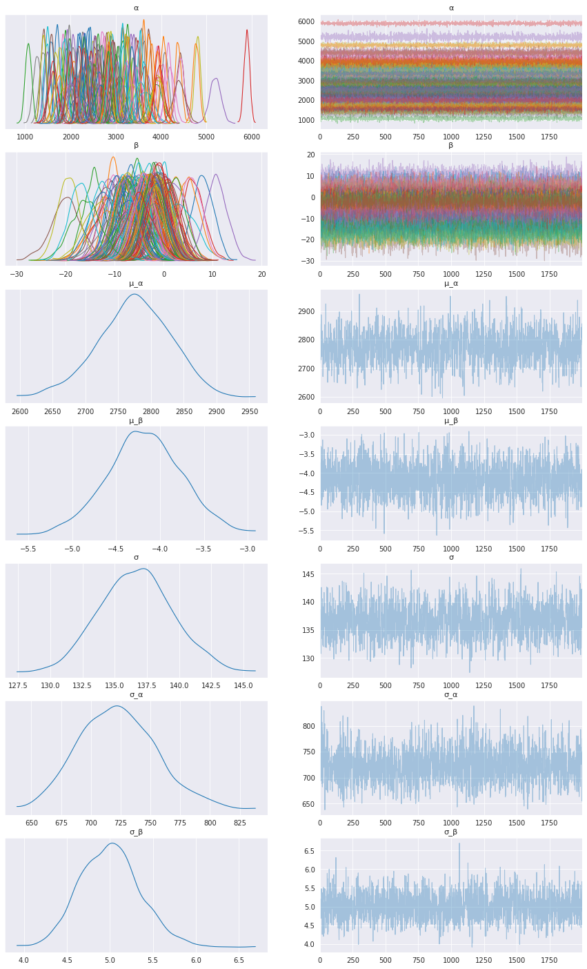
看起来我们的模型为每个患者学习到了个性化的 alpha 和 beta！

4.2. 可视化部分患者的 FVC 下降曲线

现在，让我们直观地检查模型预测的 FVC 下降曲线。我们将完整填写 FVC 表格，预测所有缺失值。第一步是创建一个要填充的表格

def create_prediction_template(unique_patient_df, weeks_series):
    unique_patient_df["_temp"] = True
    weeks = pd.DataFrame(weeks_series, columns=["Weeks"])
    weeks["_temp"] = True
    return unique_patient_df.merge(weeks, on="_temp").drop(["_temp"], axis=1)

patients = train[["Patient", "patient_code"]].drop_duplicates()
start_week_number = -12
end_week_number = 134
predict_weeks = pd.Series(np.arange(start_week_number, end_week_number))
pred_template = create_prediction_template(patients, predict_weeks)

预测 FVC 表格中的缺失值以及每个值的置信度 (sigma) 变得非常容易

patient_code = pred_template["patient_code"].values
Weeks = pred_template["Weeks"].values
predictive = Predictive(model, posterior_samples, return_sites=["σ", "obs"])
samples_predictive = predictive(random.PRNGKey(0), patient_code, Weeks, None)

请注意，为了使 `Predictive <https://num.pyro.org.cn/en/stable/utilities.html#numpyro.infer.util.Predictive>`__ 正常工作，模型的响应变量（在本例中为 FVC_obs）必须设置为 None。

现在，让我们将预测值与真实值放在一起，以便可视化它们

df = pred_template.copy()
df["FVC_pred"] = samples_predictive["obs"].T.mean(axis=1)
df["sigma"] = samples_predictive["obs"].T.std(axis=1)
df["FVC_inf"] = df["FVC_pred"] - df["sigma"]
df["FVC_sup"] = df["FVC_pred"] + df["sigma"]
df = pd.merge(
    df, train[["Patient", "Weeks", "FVC"]], how="left", on=["Patient", "Weeks"]
)
df = df.rename(columns={"FVC": "FVC_true"})
df.head()

	患者	患者代码	周	FVC_预测值	sigma	FVC_下限	FVC_上限	FVC_真实值
0	ID00007637202177411956430	0	-12	2226.545166	160.158493	2066.386719	2386.703613	NaN
1	ID00007637202177411956430	0	-11	2216.172852	160.390778	2055.781982	2376.563721	NaN
2	ID00007637202177411956430	0	-10	2219.136963	155.339615	2063.797363	2374.476562	NaN
3	ID00007637202177411956430	0	-9	2214.727051	153.333313	2061.393799	2368.060303	NaN
4	ID00007637202177411956430	0	-8	2208.758545	157.368637	2051.389893	2366.127197	NaN

最后，让我们看看对 3 名患者的预测

def chart_patient_with_predictions(patient_id, ax):
    data = df[df["Patient"] == patient_id]
    x = data["Weeks"]
    ax.set_title(patient_id)
    ax.plot(x, data["FVC_true"], "o")
    ax.plot(x, data["FVC_pred"])
    ax = sns.regplot(x=x, y=data["FVC_true"], ax=ax, ci=None, line_kws={"color": "red"})
    ax.fill_between(x, data["FVC_inf"], data["FVC_sup"], alpha=0.5, color="#ffcd3c")
    ax.set_ylabel("FVC")


f, axes = plt.subplots(1, 3, figsize=(15, 5))
chart_patient_with_predictions("ID00007637202177411956430", axes[0])
chart_patient_with_predictions("ID00009637202177434476278", axes[1])
chart_patient_with_predictions("ID00011637202177653955184", axes[2])

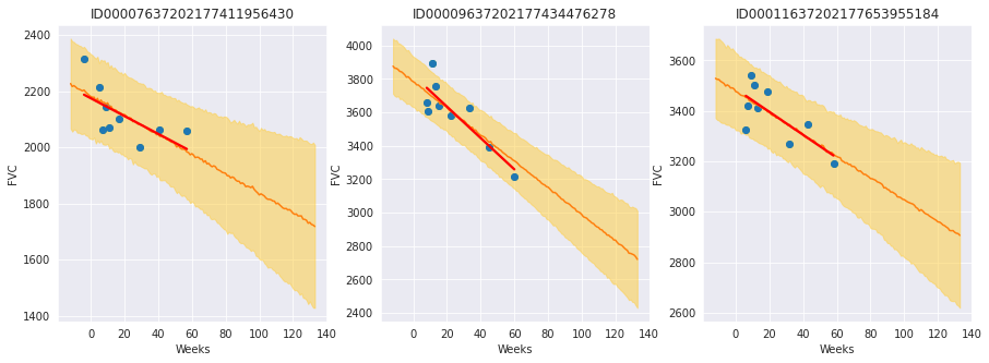
结果与我们预期完全一致！重点观察

• 模型充分学习了贝叶斯线性回归！橙色线（学习到的预测 FVC 均值）与红色线（确定性线性回归）非常吻合。但最重要的是：它学会了预测不确定性，如浅橙色区域所示（FVC 均值线上方和下方一个 sigma 范围）

• 模型在数据点更分散的地方（第 1 和第 3 位患者）预测的不确定性更高。相反，在数据点更密集的地方（第 2 位患者），模型预测的置信度更高（浅橙色区域更窄）

• 最后，在所有患者中，我们可以看到随着时间推移不确定性增加：随着周数增加，浅橙色区域变宽！

4.3. 计算修改后的拉普拉斯对数似然和 RMSE

如前所述，竞赛是根据拉普拉斯对数似然的修改版本进行评估的。在医疗应用中，评估模型对其决策的置信度非常有用。因此，该指标旨在反映每次预测的准确性和确定性。

对于每个真实的 FVC 测量值，我们预测了 FVC 和置信度度量（标准差 \(\sigma\)）。指标计算如下

\begin{align} \sigma_{clipped} &= max(\sigma, 70) \\ \delta &= min(|FVC_{true} - FVC_{pred}|, 1000) \\ metric &= -\dfrac{\sqrt{2}\delta}{\sigma_{clipped}} - \ln(\sqrt{2} \sigma_{clipped}) \end{align}

误差阈值为 1000 毫升，以避免大的误差对结果产生不利影响，而置信度值被截断为 70 毫升，以反映 FVC 的近似测量不确定性。最终得分是通过对所有（患者，周）对的指标进行平均计算得出的。请注意，指标值为负，值越高越好。

接下来，我们计算指标和 RMSE

y = df.dropna()
rmse = ((y["FVC_pred"] - y["FVC_true"]) ** 2).mean() ** (1 / 2)
print(f"RMSE: {rmse:.1f} ml")

sigma_c = y["sigma"].values
sigma_c[sigma_c < 70] = 70
delta = (y["FVC_pred"] - y["FVC_true"]).abs()
delta[delta > 1000] = 1000
lll = -np.sqrt(2) * delta / sigma_c - np.log(np.sqrt(2) * sigma_c)
print(f"Laplace Log Likelihood: {lll.mean():.4f}")

RMSE: 122.3 ml
Laplace Log Likelihood: -6.1406

这些数字意味着什么？这意味着如果你采用这种方法，你将在比赛中超越大多数公开的解决方案。奇怪的是，绝大多数公开的解决方案采用了标准的确定性神经网络，通过分位数损失来建模不确定性。大多数人仍然采用频率派方法。

不确定性对于单一预测在机器学习中变得越来越重要，并且经常是必需的。尤其当错误预测的后果很严重时，我们需要知道个体预测的概率分布是什么。举例来说，Kaggle 刚刚推出了 Lyft 赞助的一项新竞赛，旨在为自动驾驶车辆构建运动预测模型。“我们要求您预测每个智能体的几条轨迹，并为每条轨迹提供置信度分数。”

5. 向模型层次添加一层：吸烟状态

我们可以通过将 SmokingStatus 列作为汇集层来扩展模型，其中模型参数将按“从不吸烟”、“前吸烟者”和“目前吸烟”这几个组进行部分汇集。为此，我们需要

1. 对 SmokingStatus 列进行编码

2. 将患者编码映射到吸烟状态编码

3. 使用附加的层次结构细化并重新训练模型

train["SmokingStatus"].value_counts()

Ex-smoker           1038
Never smoked         429
Currently smokes      82
Name: SmokingStatus, dtype: int64

patient_code = train["patient_code"].values
Weeks = train["Weeks"].values

smoking_status_encoder = LabelEncoder()
train["smoking_status_code"] = smoking_status_encoder.fit_transform(
    train["SmokingStatus"]
)

smoking_status_code = train["smoking_status_code"].values

map_patient_to_smoking_status = (
    train[["patient_code", "smoking_status_code"]]
    .drop_duplicates()
    .set_index("patient_code", verify_integrity=True)
    .sort_index()["smoking_status_code"]
    .values
)

def model_smoking_hierarchy(
    patient_code, Weeks, map_patient_to_smoking_status, FVC_obs=None
):
    μ_α_global = numpyro.sample("μ_α_global", dist.Normal(0.0, 500.0))
    σ_α_global = numpyro.sample("σ_α_global", dist.HalfNormal(100.0))
    μ_β_global = numpyro.sample("μ_β_global", dist.Normal(0.0, 3.0))
    σ_β_global = numpyro.sample("σ_β_global", dist.HalfNormal(3.0))

    n_patients = len(np.unique(patient_code))
    n_smoking_statuses = len(np.unique(map_patient_to_smoking_status))

    with numpyro.plate("plate_smoking_status", n_smoking_statuses):
        μ_α_smoking_status = numpyro.sample(
            "μ_α_smoking_status", dist.Normal(μ_α_global, σ_α_global)
        )
        μ_β_smoking_status = numpyro.sample(
            "μ_β_smoking_status", dist.Normal(μ_β_global, σ_β_global)
        )

    with numpyro.plate("plate_i", n_patients):
        α = numpyro.sample(
            "α",
            dist.Normal(μ_α_smoking_status[map_patient_to_smoking_status], σ_α_global),
        )
        β = numpyro.sample(
            "β",
            dist.Normal(μ_β_smoking_status[map_patient_to_smoking_status], σ_β_global),
        )

    σ = numpyro.sample("σ", dist.HalfNormal(100.0))
    FVC_est = α[patient_code] + β[patient_code] * Weeks

    with numpyro.plate("data", len(patient_code)):
        numpyro.sample("obs", dist.Normal(FVC_est, σ), obs=FVC_obs)

对模型进行重新参数化

分层模型通常需要进行重新参数化，以便 MCMC 能够探索完整的参数空间。下面使用 NumPyro 的 LocScaleReparam 来实现这一点。更多详细信息请参阅bad_posterior_geometry.ipynb 和 funnel.py。Thomas Wiecki 还有一篇关于开发非中心化模型的精彩博文。

from numpyro.handlers import reparam
from numpyro.infer.reparam import LocScaleReparam

reparam_config = {
    "μ_α_smoking_status": LocScaleReparam(0),
    "μ_β_smoking_status": LocScaleReparam(0),
    "α": LocScaleReparam(0),
    "β": LocScaleReparam(0),
}
reparam_model_smoking_hierarchy = reparam(
    model_smoking_hierarchy, config=reparam_config
)

nuts_kernel = NUTS(reparam_model_smoking_hierarchy, target_accept_prob=0.97)

mcmc = MCMC(nuts_kernel, num_samples=3000, num_warmup=5000)
rng_key = random.PRNGKey(0)
mcmc.run(rng_key, patient_code, Weeks, map_patient_to_smoking_status, FVC_obs=FVC_obs)

posterior_samples = mcmc.get_samples()

sample: 100%|█████████████████████████████████| 8000/8000 [03:55<00:00, 33.99it/s, 1023 steps of size 5.68e-03. acc. prob=0.97]

5.1. 检查学习到的参数

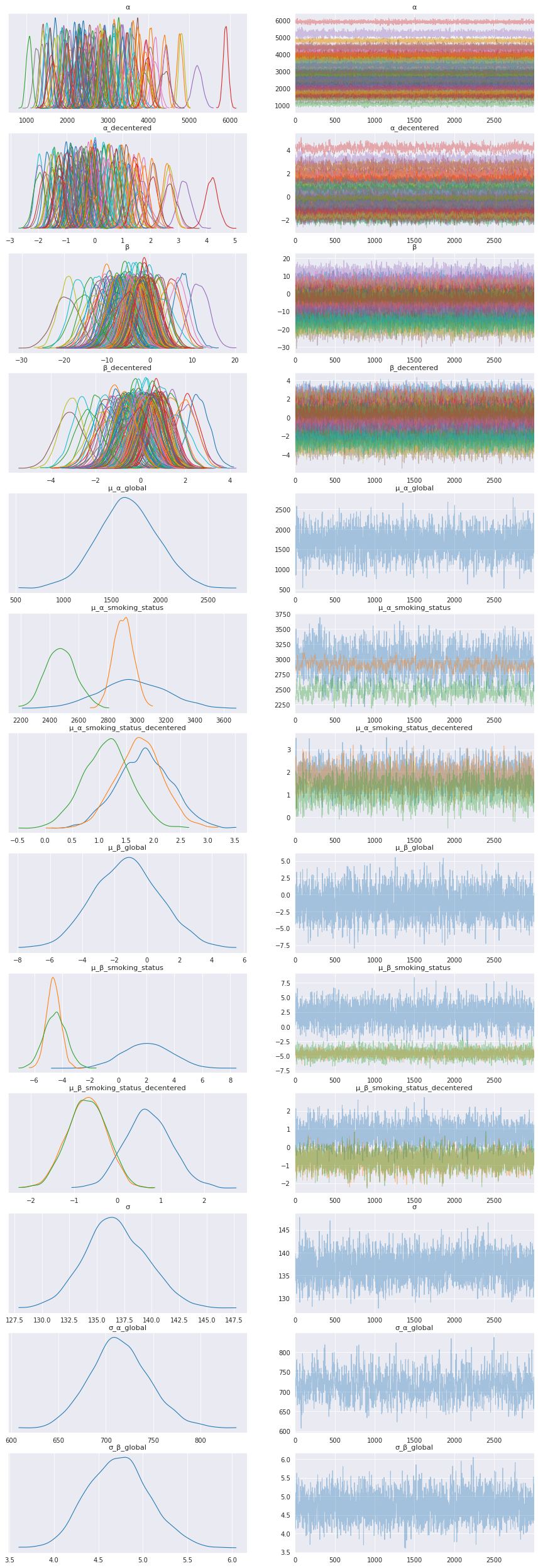
data = az.from_numpyro(mcmc)
az.plot_trace(data, compact=True, figsize=(15, 45));

吸烟状态分布

添加吸烟状态分布图例，以帮助解释该层次的模型结果。

吸烟状态	代码
目前吸烟	0
前吸烟者	1
从不吸烟	2

# Check the label code for each SmokingStatus
smoking_status_encoder.inverse_transform([0, 1, 2])

array(['Currently smokes', 'Ex-smoker', 'Never smoked'], dtype=object)

axes = az.plot_trace(
    data,
    var_names=["μ_α_smoking_status", "μ_β_smoking_status"],
    legend=True,
    compact=True,
    figsize=(15, 15),
)
# The legend handles were not working for the first plot
axes[0, 0].legend();

WARNING:matplotlib.legend:No artists with labels found to put in legend.  Note that artists whose label start with an underscore are ignored when legend() is called with no argument.

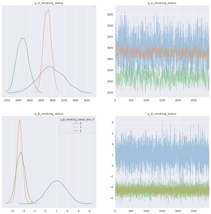
解释吸烟状态模型参数

每种吸烟状态的模型参数显示出有趣的结果，特别是趋势参数 μ_β_smoking_status。在上面的轨迹图和下面的摘要表中，目前吸烟者的趋势 μ_β_smoking_status[0] 具有正均值，而前吸烟者和从不吸烟者的趋势分别为负值，即 μ_β_smoking_status[1] 和 μ_β_smoking_status[2]。

trace = az.from_numpyro(mcmc)
az.summary(
    trace,
    var_names=["μ_α_global", "μ_β_global", "μ_α_smoking_status", "μ_β_smoking_status"],
)

Shape validation failed: input_shape: (1, 3000), minimum_shape: (chains=2, draws=4)

	均值	标准差	hdi_3%	hdi_97%	mcse_均值	mcse_标准差	ess_整体	ess_尾部	r_hat
μ_α_全局	1660.172	309.657	1118.038	2274.933	6.589	4.660	2203.0	2086.0	NaN
μ_β_全局	-1.252	2.062	-5.014	2.678	0.037	0.035	3040.0	2041.0	NaN
μ_α_吸烟状态[0]	2970.486	227.761	2572.943	3429.343	7.674	5.452	878.0	1416.0	NaN
μ_α_吸烟状态[1]	2907.950	68.011	2782.993	3035.172	5.209	3.698	171.0	281.0	NaN
μ_α_吸烟状态[2]	2475.281	102.948	2286.072	2671.298	6.181	4.381	278.0	566.0	NaN
μ_β_吸烟状态[0]	2.061	1.713	-1.278	5.072	0.032	0.024	2797.0	2268.0	NaN
μ_β_吸烟状态[1]	-4.625	0.498	-5.566	-3.721	0.010	0.007	2309.0	2346.0	NaN
μ_β_吸烟状态[2]	-4.513	0.789	-6.011	-3.056	0.016	0.011	2466.0	2494.0	NaN

让我们看看这些个体患者的曲线，以帮助解释这些模型结果。

5.2. 可视化部分患者的 FVC 下降曲线

patient_code = pred_template["patient_code"].values
Weeks = pred_template["Weeks"].values
predictive = Predictive(
    reparam_model_smoking_hierarchy, posterior_samples, return_sites=["σ", "obs"]
)
samples_predictive = predictive(
    random.PRNGKey(0), patient_code, Weeks, map_patient_to_smoking_status, None
)

df = pred_template.copy()
df["FVC_pred"] = samples_predictive["obs"].T.mean(axis=1)
df["sigma"] = samples_predictive["obs"].T.std(axis=1)
df["FVC_inf"] = df["FVC_pred"] - df["sigma"]
df["FVC_sup"] = df["FVC_pred"] + df["sigma"]
df = pd.merge(
    df, train[["Patient", "Weeks", "FVC"]], how="left", on=["Patient", "Weeks"]
)
df = df.rename(columns={"FVC": "FVC_true"})
df.head()

	患者	患者代码	周	FVC_预测值	sigma	FVC_下限	FVC_上限	FVC_真实值
0	ID00007637202177411956430	0	-12	2229.098877	157.880753	2071.218018	2386.979736	NaN
1	ID00007637202177411956430	0	-11	2225.022461	157.358429	2067.664062	2382.380859	NaN
2	ID00007637202177411956430	0	-10	2224.487549	155.416016	2069.071533	2379.903564	NaN
3	ID00007637202177411956430	0	-9	2212.780518	154.162155	2058.618408	2366.942627	NaN
4	ID00007637202177411956430	0	-8	2219.202393	154.729507	2064.472900	2373.931885	NaN

f, axes = plt.subplots(1, 3, figsize=(15, 5))
chart_patient_with_predictions("ID00048637202185016727717", axes[0])  # Never smoked
chart_patient_with_predictions("ID00342637202287526592911", axes[1])  # Ex-smoker
chart_patient_with_predictions("ID00331637202286306023714", axes[2])  # Currently smokes

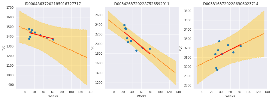
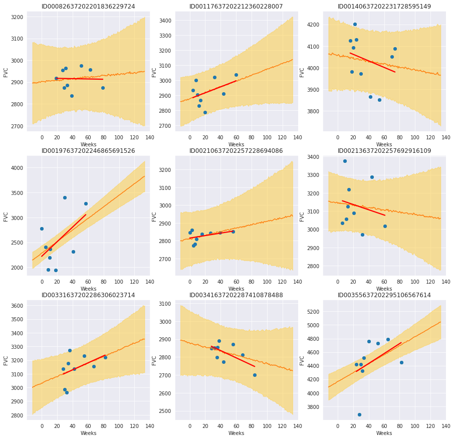
回顾目前吸烟的患者

通过绘制吸烟状态为“目前吸烟”的每位患者，我们看到一些患者具有明显的正向趋势，而另一些则没有明显趋势或呈负向趋势。趋势线比不汇集趋势线更不容易过拟合，并且在斜率和截距上显示出相对较大的不确定性。根据模型的用例，我们可以采用不同的方式进行下去

• 如果我们只是想了解不同属性与患者 FVC 随时间变化的关系，我们可以在这里停下来，得出这样的认识：在监测肺纤维化时，目前吸烟者的 FVC 可能随时间增加。我们可以对这一观察结果提出假设，并设计新的实验来检验该假设。

• 如果我们想开发一个用于治疗患者的预测模型，那么我们需要确保模型不过拟合，以便我们可以信任模型在新患者上的表现。我们可以调整模型参数，使“目前吸烟”组的模型参数更接近全局参数，甚至将该组与“前吸烟者”组合。我们可以考虑收集更多关于目前吸烟者的数据，以帮助确保模型不过拟合。

f, axes = plt.subplots(3, 3, figsize=(15, 15))
for i, patient in enumerate(
    train[train["SmokingStatus"] == "Currently smokes"]["Patient"].unique()
):
    chart_patient_with_predictions(patient, axes.flatten()[i])

5.3 包含吸烟状态层模型的修改后拉普拉斯对数似然和 RMSE

我们计算更新后模型的指标并与原始模型进行比较。

y = df.dropna()
rmse = ((y["FVC_pred"] - y["FVC_true"]) ** 2).mean() ** (1 / 2)
print(f"RMSE: {rmse:.1f} ml")

sigma_c = y["sigma"].values
sigma_c[sigma_c < 70] = 70
delta = (y["FVC_pred"] - y["FVC_true"]).abs()
delta[delta > 1000] = 1000
lll = -np.sqrt(2) * delta / sigma_c - np.log(np.sqrt(2) * sigma_c)
print(f"Laplace Log Likelihood: {lll.mean():.4f}")

RMSE: 122.6 ml
Laplace Log Likelihood: -6.1420

拉普拉斯对数似然和 RMSE 都显示吸烟状态模型的性能略差。我们了解到，直接添加这个层次并没有提高模型性能，但我们确实从吸烟状态层次中发现了一些值得深入研究的有趣结果。此外，我们可以尝试调整先验或尝试不同的层次（例如性别）来提高模型性能。

总结

最后，我希望 Pyro/NumPyro 开发者的出色工作能够帮助普及贝叶斯方法，赋予不断壮大的研究人员和实践者群体创建模型的能力，这些模型不仅可以生成预测，还可以评估预测的不确定性。

参考文献

1. Ghahramani, Z. 概率机器学习与人工智能. Nature 521, 452–459 (2015). https://doi.org/10.1038/nature14541

2. Rainforth, Thomas William Gamlen. 使用概率编程自动化推断、学习和设计。牛津大学，2017 年。