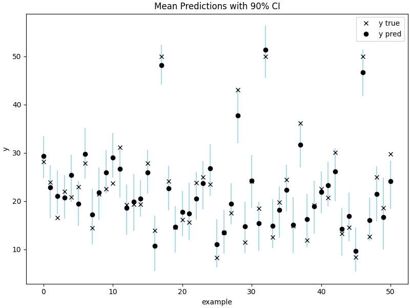
示例：使用 SteinVI 的贝叶斯神经网络

我们演示了如何使用 SteinVI 结合 BNN 预测 UCI 回归基准数据集中的波士顿房价。

import argparse
from collections import namedtuple
import datetime
from functools import partial
from time import time

from matplotlib.collections import LineCollection
import matplotlib.pyplot as plt
import numpy as np
from sklearn.model_selection import train_test_split

from jax import config, nn, numpy as jnp, random

import numpyro
from numpyro import deterministic, plate, sample, set_platform, subsample
from numpyro.contrib.einstein import MixtureGuidePredictive, RBFKernel, SteinVI
from numpyro.distributions import Gamma, Normal
from numpyro.examples.datasets import BOSTON_HOUSING, load_dataset
from numpyro.infer.autoguide import AutoNormal
from numpyro.optim import Adagrad

DataState = namedtuple("data", ["xtr", "xte", "ytr", "yte"])


def load_data() -> DataState:
    _, fetch = load_dataset(BOSTON_HOUSING, shuffle=False)
    x, y = fetch()
    xtr, xte, ytr, yte = train_test_split(x, y, train_size=0.90, random_state=1)

    return DataState(*map(partial(jnp.array, dtype=float), (xtr, xte, ytr, yte)))


def normalize(val, mean=None, std=None):
    """Normalize data to zero mean, unit variance"""
    if mean is None and std is None:
        # Only use training data to estimate mean and std.
        std = jnp.std(val, 0, keepdims=True)
        std = jnp.where(std == 0, 1.0, std)
        mean = jnp.mean(val, 0, keepdims=True)
    return (val - mean) / std, mean, std


def model(x, y=None, hidden_dim=50, sub_size=100):
    """BNN described in section 5 of [1].

    **References:**
        1. *Stein Variational Gradient Descent: A General Purpose Bayesian Inference Algorithm*
        Qiang Liu and Dilin Wang (2016).
    """

    prec_nn = sample(
        "prec_nn", Gamma(1.0, 0.1)
    )  # hyper prior for precision of nn weights and biases

    n, m = x.shape

    with plate("l1_hidden", hidden_dim, dim=-1):
        # prior l1 bias term
        b1 = sample(
            "nn_b1",
            Normal(
                0.0,
                1.0 / jnp.sqrt(prec_nn),
            ),
        )
        assert b1.shape == (hidden_dim,)

        with plate("l1_feat", m, dim=-2):
            w1 = sample(
                "nn_w1", Normal(0.0, 1.0 / jnp.sqrt(prec_nn))
            )  # prior on l1 weights
            assert w1.shape == (m, hidden_dim)

    with plate("l2_hidden", hidden_dim, dim=-1):
        w2 = sample(
            "nn_w2", Normal(0.0, 1.0 / jnp.sqrt(prec_nn))
        )  # prior on output weights

    b2 = sample(
        "nn_b2", Normal(0.0, 1.0 / jnp.sqrt(prec_nn))
    )  # prior on output bias term

    # precision prior on observations
    prec_obs = sample("prec_obs", Gamma(1.0, 0.1))

    with plate("data", x.shape[0], subsample_size=sub_size, dim=-1):
        batch_x = subsample(x, event_dim=1)
        if y is not None:
            batch_y = subsample(y, event_dim=0)
        else:
            batch_y = y

        loc_y = deterministic("y_bnn", nn.relu(batch_x @ w1 + b1) @ w2 + b2)

        sample(
            "y",
            Normal(
                loc_y, 1.0 / jnp.sqrt(prec_obs)
            ),  # 1 hidden layer with ReLU activation
            obs=batch_y,
        )


def main(args):
    data = load_data()

    inf_key, pred_key, data_key = random.split(random.PRNGKey(args.rng_key), 3)
    # Normalize features to zero mean unit variance.
    x, xtr_mean, xtr_std = normalize(data.xtr)

    rng_key, inf_key = random.split(inf_key)

    guide = AutoNormal(model)

    stein = SteinVI(
        model,
        guide,
        Adagrad(1.0),
        RBFKernel(),
        repulsion_temperature=args.repulsion,
        num_stein_particles=args.num_stein_particles,
        num_elbo_particles=args.num_elbo_particles,
    )
    start = time()

    # Use keyword params for static (shape etc.)
    result = stein.run(
        rng_key,
        args.max_iter,
        x,
        data.ytr,
        hidden_dim=args.hidden_dim,
        sub_size=args.subsample_size,
        progress_bar=args.progress_bar,
    )
    time_taken = time() - start

    pred = MixtureGuidePredictive(
        model,
        guide=stein.guide,
        params=stein.get_params(result.state),
        num_samples=100,
        guide_sites=stein.guide_sites,
    )
    xte, _, _ = normalize(
        data.xte, xtr_mean, xtr_std
    )  # Use train data statistics when accessing generalization.
    n = xte.shape[0]

    pred_y = pred(pred_key, xte, sub_size=n, hidden_dim=args.hidden_dim)["y"]
    rmse = jnp.sqrt(jnp.mean((pred_y.mean(0) - data.yte) ** 2))

    print(rf"Time taken: {datetime.timedelta(seconds=int(time_taken))}")
    print(rf"RMSE: {rmse:.2f}")

    # Compute mean prediction and confidence interval around median
    percentiles = jnp.percentile(pred_y, jnp.array([5.0, 95.0]), axis=0)

    # Make plots
    fig, ax = plt.subplots(figsize=(8, 6), constrained_layout=True)
    ran = np.arange(pred_y.shape[1])
    ax.add_collection(
        LineCollection(
            zip(zip(ran, percentiles[0]), zip(ran, percentiles[1])), colors="lightblue"
        )
    )
    ax.plot(data.yte, "kx", label="y true")
    ax.plot(pred_y.mean(0), "ko", label="y pred")
    ax.set(xlabel="example", ylabel="y", title="Mean Predictions with 90% CI")
    ax.legend()
    fig.savefig("stein_bnn.pdf")


if __name__ == "__main__":
    assert numpyro.__version__.startswith("0.18.0")
    config.update("jax_debug_nans", True)

    parser = argparse.ArgumentParser()
    parser.add_argument("--subsample-size", type=int, default=100)
    parser.add_argument("--max-iter", type=int, default=1000)
    parser.add_argument("--repulsion", type=float, default=1.0)
    parser.add_argument("--verbose", type=bool, default=True)
    parser.add_argument("--num-elbo-particles", type=int, default=50)
    parser.add_argument("--num-stein-particles", type=int, default=5)
    parser.add_argument("--progress-bar", type=bool, default=True)
    parser.add_argument("--rng-key", type=int, default=142)
    parser.add_argument("--device", default="cpu", choices=["gpu", "cpu"])
    parser.add_argument("--hidden-dim", default=50, type=int)

    args = parser.parse_args()

    set_platform(args.device)

    main(args)