交互式在线版本：

贝叶斯分层叠加：水井切换案例研究

摄影：Belinda Fewings，https://unsplash.com/photos/6p-KtXCBGNw。

目录

• 引言

• 1. 探索性数据分析

• 2. 准备 6 个不同的模型

  • 2.1 特征工程

  • 2.2 训练

  • 2.3 估计每个训练点的留一交叉验证得分

• 3. 贝叶斯分层叠加

  • 3.1 准备叠加数据集

  • 3.2 定义叠加模型

• 4. 在测试集上评估

  • 4.1 叠加预测

  • 4.2 比较方法

• 结论

• 参考文献

引言

假设您刚刚为一个数据集拟合了 6 个模型，并且需要选择使用哪个模型来对测试集进行预测。您如何选择使用哪个模型？一些常见的策略是

• 基于交叉验证选择最佳模型；

• 平均模型，使用基于交叉验证得分的权重。

在论文《Bayesian hierarchical stacking: Some models are (somewhere) useful》（贝叶斯分层叠加：有些模型（在某些地方）有用）中，引入了一种新技术：根据输入数据，基于分层结构，使用允许变化的权重对模型进行平均。

在这里，我们将实现该论文中的第一个案例研究——尽管如此，我们仍鼓励读者查阅原始论文，以找到其他案例研究以及理论结果。文章（R / Stan 代码）可以在此处找到。

!pip install -q numpyro@git+https://github.com/pyro-ppl/numpyro

import os

import arviz as az
from IPython.display import set_matplotlib_formats
import matplotlib.pyplot as plt
import numpy as np
import pandas as pd
from scipy.interpolate import BSpline
import seaborn as sns

import jax
import jax.numpy as jnp

import numpyro
import numpyro.distributions as dist

plt.style.use("seaborn")
if "NUMPYRO_SPHINXBUILD" in os.environ:
    set_matplotlib_formats("svg")

numpyro.set_host_device_count(4)
assert numpyro.__version__.startswith("0.18.0")

%matplotlib inline

1. 探索性数据分析

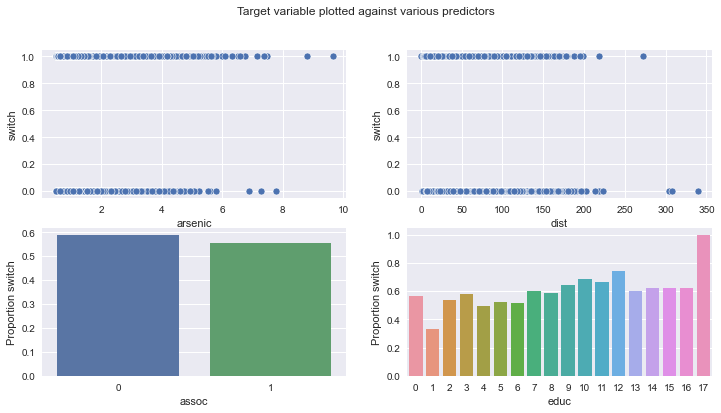
我们要处理的数据涉及孟加拉国的家庭，其中一些家庭的水中砷含量很高。受影响的家庭会想改用邻居的水井吗？

我们将数据分成训练集和测试集，然后训练六个不同的模型来尝试预测家庭是否会更换水井。接着，我们将看看在对测试集进行预测时如何对它们进行叠加！

但首先，让我们加载并可视化它！每一行代表一个家庭，我们可用的特征有

• switch：家庭是否换到另一口水井；

• arsenic：饮用水中的砷含量；

• educ：“户主”的受教育水平；

• dist100：到最近安全饮用水井的距离；

• assoc：家庭是否参与任何社区活动。

wells = pd.read_csv(
    "http://stat.columbia.edu/~gelman/arm/examples/arsenic/wells.dat", sep=" "
)

wells.head()

	switch	arsenic	dist	assoc	educ
1	1	2.36	16.826000	0	0
2	1	0.71	47.321999	0	0
3	0	2.07	20.966999	0	10
4	1	1.15	21.486000	0	12
5	1	1.10	40.874001	1	14

fig, ax = plt.subplots(2, 2, figsize=(12, 6))
fig.suptitle("Target variable plotted against various predictors")
sns.scatterplot(data=wells, x="arsenic", y="switch", ax=ax[0][0])
sns.scatterplot(data=wells, x="dist", y="switch", ax=ax[0][1])
sns.barplot(
    data=wells.groupby("assoc")["switch"].mean().reset_index(),
    x="assoc",
    y="switch",
    ax=ax[1][0],
)
ax[1][0].set_ylabel("Proportion switch")
sns.barplot(
    data=wells.groupby("educ")["switch"].mean().reset_index(),
    x="educ",
    y="switch",
    ax=ax[1][1],
)
ax[1][1].set_ylabel("Proportion switch");

接下来，我们将选择 200 个观测值作为我们的训练集的一部分，以及 1500 个观测值作为我们的测试集的一部分。

np.random.seed(1)
train_id = wells.sample(n=200).index
test_id = wells.loc[~wells.index.isin(train_id)].sample(n=1500).index
y_train = wells.loc[train_id, "switch"].to_numpy()
y_test = wells.loc[test_id, "switch"].to_numpy()

2. 准备 6 个不同的候选模型

2.1 特征工程

首先，让我们添加几个新列

• edu0：educ 是否为 0，

• edu1：educ 是否在 1 到 5 之间，

• edu2：educ 是否在 6 到 11 之间，

• edu3：educ 是否在 12 到 17 之间，

• logarsenic：arsenic 的自然对数，

• assoc_half：assoc 的一半，

• as_square：arsenic 的自然对数的平方，

• as_third：arsenic 的自然对数的立方，

• dist100：dist 除以 100，

• intercept：只是一个由 1 组成的列。

我们将首先为训练集拟合 6 个不同的模型

• 使用 intercept、arsenic、assoc、edu1、edu2 和 edu3 的逻辑回归；

• 与上面相同，但用 logarsenic 代替 arsenic；

• 与第一个相同，但同时包含平方和立方特征；

• 与第一个相同，但同时包含从 logarsenic 导出的样条特征；

• 与第一个相同，但同时包含从 dist100 导出的样条特征；

• 与第一个相同，但用 educ 代替二元 edu 变量。

wells["edu0"] = wells["educ"].isin(np.arange(0, 1)).astype(int)
wells["edu1"] = wells["educ"].isin(np.arange(1, 6)).astype(int)
wells["edu2"] = wells["educ"].isin(np.arange(6, 12)).astype(int)
wells["edu3"] = wells["educ"].isin(np.arange(12, 18)).astype(int)
wells["logarsenic"] = np.log(wells["arsenic"])
wells["assoc_half"] = wells["assoc"] / 2.0
wells["as_square"] = wells["logarsenic"] ** 2
wells["as_third"] = wells["logarsenic"] ** 3
wells["dist100"] = wells["dist"] / 100.0
wells["intercept"] = 1

def bs(x, knots, degree):
    """
    Generate the B-spline basis matrix for a polynomial spline.

    Parameters
    ----------
    x
        predictor variable.
    knots
        locations of internal breakpoints (not padded).
    degree
        degree of the piecewise polynomial.

    Returns
    -------
    pd.DataFrame
        Spline basis matrix.

    Notes
    -----
    This mirrors ``bs`` from splines package in R.
    """
    padded_knots = np.hstack(
        [[x.min()] * (degree + 1), knots, [x.max()] * (degree + 1)]
    )
    return pd.DataFrame(
        BSpline(padded_knots, np.eye(len(padded_knots) - degree - 1), degree)(x)[:, 1:],
        index=x.index,
    )


knots = np.quantile(wells.loc[train_id, "logarsenic"], np.linspace(0.1, 0.9, num=10))
spline_arsenic = bs(wells["logarsenic"], knots=knots, degree=3)
knots = np.quantile(wells.loc[train_id, "dist100"], np.linspace(0.1, 0.9, num=10))
spline_dist = bs(wells["dist100"], knots=knots, degree=3)

features_0 = ["intercept", "dist100", "arsenic", "assoc", "edu1", "edu2", "edu3"]
features_1 = ["intercept", "dist100", "logarsenic", "assoc", "edu1", "edu2", "edu3"]
features_2 = [
    "intercept",
    "dist100",
    "arsenic",
    "as_third",
    "as_square",
    "assoc",
    "edu1",
    "edu2",
    "edu3",
]
features_3 = ["intercept", "dist100", "assoc", "edu1", "edu2", "edu3"]
features_4 = ["intercept", "logarsenic", "assoc", "edu1", "edu2", "edu3"]
features_5 = ["intercept", "dist100", "logarsenic", "assoc", "educ"]

X0 = wells.loc[train_id, features_0].to_numpy()
X1 = wells.loc[train_id, features_1].to_numpy()
X2 = wells.loc[train_id, features_2].to_numpy()
X3 = (
    pd.concat([wells.loc[:, features_3], spline_arsenic], axis=1)
    .loc[train_id]
    .to_numpy()
)
X4 = pd.concat([wells.loc[:, features_4], spline_dist], axis=1).loc[train_id].to_numpy()
X5 = wells.loc[train_id, features_5].to_numpy()

X0_test = wells.loc[test_id, features_0].to_numpy()
X1_test = wells.loc[test_id, features_1].to_numpy()
X2_test = wells.loc[test_id, features_2].to_numpy()
X3_test = (
    pd.concat([wells.loc[:, features_3], spline_arsenic], axis=1)
    .loc[test_id]
    .to_numpy()
)
X4_test = (
    pd.concat([wells.loc[:, features_4], spline_dist], axis=1).loc[test_id].to_numpy()
)
X5_test = wells.loc[test_id, features_5].to_numpy()

train_x_list = [X0, X1, X2, X3, X4, X5]
test_x_list = [X0_test, X1_test, X2_test, X3_test, X4_test, X5_test]
K = len(train_x_list)

2.2 训练

每个模型将以相同的方式进行训练——使用伯努利似然和 logit 链接函数。

def logistic(x, y=None):
    beta = numpyro.sample("beta", dist.Normal(0, 3).expand([x.shape[1]]))
    logits = numpyro.deterministic("logits", jnp.matmul(x, beta))

    numpyro.sample(
        "obs",
        dist.Bernoulli(logits=logits),
        obs=y,
    )

fit_list = []
for k in range(K):
    sampler = numpyro.infer.NUTS(logistic)
    mcmc = numpyro.infer.MCMC(
        sampler, num_chains=4, num_samples=1000, num_warmup=1000, progress_bar=False
    )
    rng_key = jax.random.fold_in(jax.random.PRNGKey(13), k)
    mcmc.run(rng_key, x=train_x_list[k], y=y_train)
    fit_list.append(mcmc)

2.3 估计每个训练点的留一交叉验证得分

我们将使用 LOO 来估计留一交叉验证得分，而不是对每个模型重新拟合 100 次。

def find_point_wise_loo_score(fit):
    return az.loo(az.from_numpyro(fit), pointwise=True, scale="log").loo_i.values


lpd_point = np.vstack([find_point_wise_loo_score(fit) for fit in fit_list]).T
exp_lpd_point = np.exp(lpd_point)

3. 贝叶斯分层叠加

3.1 准备叠加数据集

为了确定叠加权重如何在训练集和测试集之间变化，我们将需要创建包含我们希望叠加权重依赖的所有特征的“叠加数据集”。这些特征应该如何包含？对于离散特征，这很简单，我们只需对其进行独热编码。但对于连续特征，我们需要一个技巧。在方程 (16) 中，作者建议如下：如果您有一个连续特征 f，则用以下两个特征替换它

• f_l：f 减去 f 的中位数，截断到 0 以上；

• f_r：f 减去 f 的中位数，截断到 0 以下；

dist100_median = wells.loc[wells.index[train_id], "dist100"].median()
logarsenic_median = wells.loc[wells.index[train_id], "logarsenic"].median()
wells["dist100_l"] = (wells["dist100"] - dist100_median).clip(upper=0)
wells["dist100_r"] = (wells["dist100"] - dist100_median).clip(lower=0)
wells["logarsenic_l"] = (wells["logarsenic"] - logarsenic_median).clip(upper=0)
wells["logarsenic_r"] = (wells["logarsenic"] - logarsenic_median).clip(lower=0)

stacking_features = [
    "edu0",
    "edu1",
    "edu2",
    "edu3",
    "assoc_half",
    "dist100_l",
    "dist100_r",
    "logarsenic_l",
    "logarsenic_r",
]
X_stacking_train = wells.loc[train_id, stacking_features].to_numpy()
X_stacking_test = wells.loc[test_id, stacking_features].to_numpy()

3.2 定义叠加模型

我们寻求找到一个权重矩阵 \(W\)，用于乘以模型的预测结果。我们定义一个矩阵 \(Pred\)，其中 \(Pred_{i,k}\) 表示模型 \(k\) 对点 \(i\) 做出的预测。那么点 \(i\) 的最终预测将是

\[\sum_k W_{i, k}Pred_{i,k}\]

这样的矩阵 \(W\) 需要每一列的和为 \(1\)。因此，我们计算 \(W\) 的每一行 \(W_i\) 为

\[W_i = \text{softmax}(X\_\text{stacking}_i \cdot \beta),\]

其中 \(\beta\) 是我们试图确定的矩阵。对于离散特征，\(\beta\) 在可能的输入上被赋予了分层结构。另一方面，连续特征在本案例研究中没有获得分层结构，只是根据输入值进行变化。

请注意，对于离散特征，使用了非中心参数化。另请注意，我们只需估计 K-1 列的 \(\beta\)，因为对于每个 i，权重 W_{i, k} 的总和必须为 1。

def stacking(
    X,
    d_discrete,
    X_test,
    lpd_point,
    tau_mu,
    tau_sigma,
    *,
    test,
):
    """
    Get weights with which to stack candidate models' predictions.

    Parameters
    ----------
    X
        Training stacking matrix: features on which stacking weights should depend, for the
        training set.
    d_discrete
        Number of discrete features in `X` and `X_test`. The first `d_discrete` features
        from these matrices should be the discrete ones, with the continuous ones coming
        after them.
    X_test
        Test stacking matrix: features on which stacking weights should depend, for the
        testing set.
    lpd_point
        LOO score evaluated at each point in the training set, for each candidate model.
    tau_mu
        Hyperprior for mean of `beta`, for discrete features.
    tau_sigma
        Hyperprior for standard deviation of `beta`, for continuous features.
    test
        Whether to calculate stacking weights for test set.

    Notes
    -----
    Naming of variables mirrors what's used in the original paper.
    """
    N = X.shape[0]
    d = X.shape[1]
    N_test = X_test.shape[0]
    K = lpd_point.shape[1]  # number of candidate models

    with numpyro.plate("Candidate models", K - 1, dim=-2):
        # mean effect of discrete features on stacking weights
        mu = numpyro.sample("mu", dist.Normal(0, tau_mu))
        # standard deviation effect of discrete features on stacking weights
        sigma = numpyro.sample("sigma", dist.HalfNormal(scale=tau_sigma))
        with numpyro.plate("Discrete features", d_discrete, dim=-1):
            # effect of discrete features on stacking weights
            tau = numpyro.sample("tau", dist.Normal(0, 1))
        with numpyro.plate("Continuous features", d - d_discrete, dim=-1):
            # effect of continuous features on stacking weights
            beta_con = numpyro.sample("beta_con", dist.Normal(0, 1))

    # effects of features on stacking weights
    beta = numpyro.deterministic(
        "beta", jnp.hstack([(sigma.squeeze() * tau.T + mu.squeeze()).T, beta_con])
    )
    assert beta.shape == (K - 1, d)

    # stacking weights (in unconstrained space)
    f = jnp.hstack([X @ beta.T, jnp.zeros((N, 1))])
    assert f.shape == (N, K)

    # log probability of LOO training scores weighted by stacking weights.
    log_w = jax.nn.log_softmax(f, axis=1)

    # stacking weights (constrained to sum to 1)
    numpyro.deterministic("w", jnp.exp(log_w))
    logp = jax.nn.logsumexp(lpd_point + log_w, axis=1)
    numpyro.factor("logp", jnp.sum(logp))

    if test:
        # test set stacking weights (in unconstrained space)
        f_test = jnp.hstack([X_test @ beta.T, jnp.zeros((N_test, 1))])
        # test set stacking weights (constrained to sum to 1)
        numpyro.deterministic("w_test", jax.nn.softmax(f_test, axis=1))

sampler = numpyro.infer.NUTS(stacking)
mcmc = numpyro.infer.MCMC(
    sampler, num_chains=4, num_samples=1000, num_warmup=1000, progress_bar=False
)
mcmc.run(
    jax.random.PRNGKey(17),
    X=X_stacking_train,
    d_discrete=4,
    X_test=X_stacking_test,
    lpd_point=lpd_point,
    tau_mu=1.0,
    tau_sigma=0.5,
    test=True,
)
trace = mcmc.get_samples()

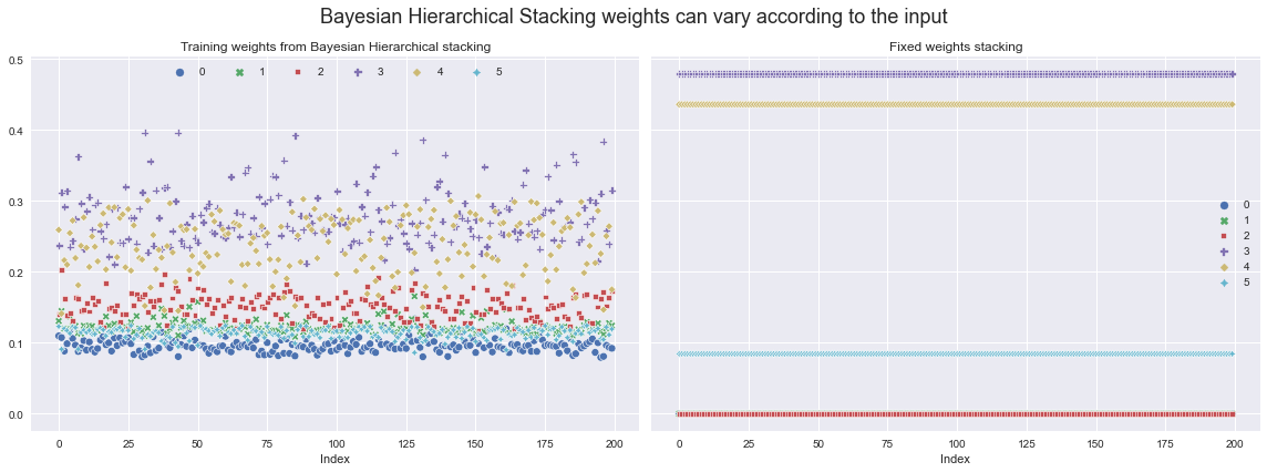
现在，我们可以从后验中提取用于对不同模型加权的权重，然后可视化它们如何在训练集上变化。

让我们将其与仅使用固定叠加权重（使用 ArviZ 计算 - 详情请参阅其文档）时的权重进行比较。

fig, ax = plt.subplots(nrows=1, ncols=2, figsize=(16, 6), sharey=True)
training_stacking_weights = trace["w"].mean(axis=0)
sns.scatterplot(data=pd.DataFrame(training_stacking_weights), ax=ax[0])
fixed_weights = (
    az.compare({idx: fit for idx, fit in enumerate(fit_list)}, method="stacking")
    .sort_index()["weight"]
    .to_numpy()
)
fixed_weights_df = pd.DataFrame(
    np.repeat(
        fixed_weights[jnp.newaxis, :],
        len(X_stacking_train),
        axis=0,
    )
)
sns.scatterplot(data=fixed_weights_df, ax=ax[1])
ax[0].set_title("Training weights from Bayesian Hierarchical stacking")
ax[1].set_title("Fixed weights stacking")
ax[0].set_xlabel("Index")
ax[1].set_xlabel("Index")
ax[0].legend(ncol=6, loc="upper center")
fig.suptitle(
    "Bayesian Hierarchical Stacking weights can vary according to the input",
    fontsize=18,
)
fig.tight_layout();

4. 在测试集上评估

4.1 叠加预测

现在，对于每个模型，让我们评估测试集中每个点的对数预测密度。一旦我们有了每个模型的预测结果，我们需要考虑如何将它们组合起来，以便为每个测试点得到一个单一的预测。

我们决定用三种方法来做这件事

• 贝叶斯分层叠加 (bhs_pred)；

• 选择训练集 LOO 得分最好的模型 (model_selection_preds)；

• 固定权重叠加 (fixed_weights_preds)。

# for each candidate model, extract the posterior predictive logits
train_preds = []
for k in range(K):
    predictive = numpyro.infer.Predictive(logistic, fit_list[k].get_samples())
    rng_key = jax.random.fold_in(jax.random.PRNGKey(19), k)
    train_pred = predictive(rng_key, x=train_x_list[k])["logits"]
    train_preds.append(train_pred.mean(axis=0))
# reshape, so we have (N, K)
train_preds = np.vstack(train_preds).T

# same as previous cell, but for test set
test_preds = []
for k in range(K):
    predictive = numpyro.infer.Predictive(logistic, fit_list[k].get_samples())
    rng_key = jax.random.fold_in(jax.random.PRNGKey(20), k)
    test_pred = predictive(rng_key, x=test_x_list[k])["logits"]
    test_preds.append(test_pred.mean(axis=0))
test_preds = np.vstack(test_preds).T

# get the stacking weights for the test set
test_stacking_weights = trace["w_test"].mean(axis=0)
# get predictions using the stacking weights
bhs_predictions = (test_stacking_weights * test_preds).sum(axis=1)
# get predictions using only the model with the best LOO score
model_selection_preds = test_preds[:, lpd_point.sum(axis=0).argmax()]
# get predictions using fixed stacking weights, dependent on the LOO score
fixed_weights_preds = (fixed_weights * test_preds).sum(axis=1)

4.2 比较方法

让我们比较测试集上的负对数预测密度得分（注意 - 越低越好）

fig, ax = plt.subplots(figsize=(12, 6))
neg_log_pred_densities = np.vstack(
    [
        -dist.Bernoulli(logits=bhs_predictions).log_prob(y_test),
        -dist.Bernoulli(logits=model_selection_preds).log_prob(y_test),
        -dist.Bernoulli(logits=fixed_weights_preds).log_prob(y_test),
    ]
).T
neg_log_pred_density = pd.DataFrame(
    neg_log_pred_densities,
    columns=[
        "Bayesian Hierarchical Stacking",
        "Model selection",
        "Fixed stacking weights",
    ],
)
sns.barplot(
    data=neg_log_pred_density.reindex(
        columns=neg_log_pred_density.mean(axis=0).sort_values(ascending=False).index
    ),
    orient="h",
    ax=ax,
)
ax.set_title(
    "Bayesian Hierarchical Stacking performs best here", fontdict={"fontsize": 18}
)
ax.set_xlabel("Negative mean log predictive density (lower is better)");

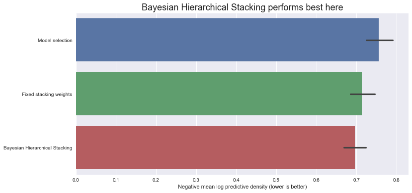
因此，在这个数据集上，采用这种特定的训练-测试划分，贝叶斯分层叠加与模型选择和固定权重叠加相比，确实带来了一点增益。

4.3 这能否证明贝叶斯分层叠加有效？

不，单次训练-测试划分不能证明任何事情。请查阅原始论文，其中包含不同训练集大小和不同训练-测试划分下的重复结果，这些结果表明贝叶斯分层叠加始终优于模型选择和固定权重叠加。

本笔记本的目标只是展示如何在 NumPyro 中实现这项技术。

结论

我们已经了解了贝叶斯分层叠加如何帮助我们以不会过拟合的方式对具有输入相关权重的模型进行平均。我们只实现了论文中的第一个案例研究，但鼓励读者也查阅其他两个案例。此外，请查阅论文，以获取理论结果和更多实验结果。

参考文献

1. Yuling Yao, Gregor Pirš, Aki Vehtari, Andrew Gelman (2021)。Bayesian hierarchical stacking: Some models are (somewhere) useful（贝叶斯分层叠加：有些模型（在某些地方）有用）

2. Måns Magnusson, Michael Riis Andersen, Johan Jonasson, Aki Vehtari (2020)。Leave-One-Out Cross-Validation for Bayesian Model Comparison in Large Data（大型数据中贝叶斯模型比较的留一交叉验证）

3. https://github.com/yao-yl/hierarchical-stacking-code.

4. Thomas Wiecki (2017)。Why hierarchical models are awesome, tricky, and Bayesian（为什么分层模型很棒、很棘手且是贝叶斯式的）