在线交互版本：

希尔伯特空间近似高斯过程模块

在此 notebook 中，我们提供了一个如何使用 希尔伯特空间高斯过程 模块的示例。我们使用一个合成数据集来说明模块中提供的一些核近似函数的用法。

备注：此示例取自原始博客文章 A Conceptual and Practical Introduction to Hilbert Space GPs Approximation Methods。

准备 Notebook

!pip install -q numpyro@git+https://github.com/pyro-ppl/numpyro arviz

import os

import arviz as az
from IPython.display import set_matplotlib_formats
import matplotlib.pyplot as plt
from matplotlib.ticker import MultipleLocator

from jax import random
import jax.numpy as jnp

import numpyro
from numpyro.contrib.hsgp.approximation import hsgp_squared_exponential
from numpyro.contrib.hsgp.laplacian import eigenfunctions
from numpyro.contrib.hsgp.spectral_densities import (
    diag_spectral_density_squared_exponential,
)
import numpyro.distributions as dist
from numpyro.infer import MCMC, NUTS, Predictive

plt.style.use("bmh")
if "NUMPYRO_SPHINXBUILD" in os.environ:
    set_matplotlib_formats("svg")

plt.rcParams["figure.figsize"] = [10, 6]

numpyro.set_host_device_count(n=4)

rng_key = random.PRNGKey(seed=42)

assert numpyro.__version__.startswith("0.18.0")

%load_ext autoreload
%autoreload 2
%config InlineBackend.figure_format = "retina"

生成合成数据

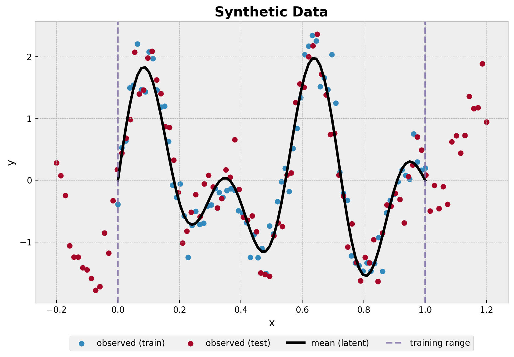
我们在一个一维空间中生成合成数据。我们将数据分成训练集和测试集。

def generate_synthetic_data(rng_key, start, stop: float, num, scale):
    x = jnp.linspace(start=start, stop=stop, num=num)
    y = jnp.sin(4 * jnp.pi * x) + jnp.sin(7 * jnp.pi * x)
    y_obs = y + scale * random.normal(rng_key, shape=(num,))
    return x, y, y_obs


n_train = 80
n_test = 100
scale = 0.3

rng_key, rng_subkey = random.split(rng_key)
x_train, y_train, y_train_obs = generate_synthetic_data(
    rng_key=rng_subkey, start=0, stop=1, num=n_train, scale=scale
)

rng_key, rng_subkey = random.split(rng_key)
x_test, y_test, y_test_obs = generate_synthetic_data(
    rng_key=rng_subkey, start=-0.2, stop=1.2, num=n_test, scale=scale
)

fig, ax = plt.subplots()
ax.scatter(x_train, y_train_obs, c="C0", label="observed (train)")
ax.scatter(x_test, y_test_obs, c="C1", label="observed (test)")
ax.plot(x_train, y_train, color="black", linewidth=3, label="mean (latent)")
ax.axvline(x=0, color="C2", alpha=0.8, linestyle="--", linewidth=2)
ax.axvline(
    x=1, color="C2", linestyle="--", alpha=0.8, linewidth=2, label="training range"
)
ax.legend(loc="upper center", bbox_to_anchor=(0.5, -0.1), ncol=4)
ax.set(xlabel="x", ylabel="y")
ax.set_title("Synthetic Data", fontsize=16, fontweight="bold");

建议在使用近似函数之前对数据进行中心化。

train_mean = x_train.mean()
x_train_centered = x_train - train_mean
x_test_centered = x_test - train_mean

指定模型

现在我们指定模型。我们将使用平方指数核函数来建模高斯似然的均值。此核函数依赖于两个参数：

• 幅度 alpha。

• 长度尺度 length。

对于这两个参数，我们需要指定先验分布。

接下来，我们使用函数 hsgp_squared_exponential 用基函数来近似核函数。我们需要指定是否要使用线性模型近似的 centered 或 non-centered 参数化。

def model(x, ell, m, non_centered, y=None):
    # --- Priors ---
    alpha = numpyro.sample("alpha", dist.InverseGamma(concentration=12, rate=10))
    length = numpyro.sample("length", dist.InverseGamma(concentration=6, rate=1))
    noise = numpyro.sample("noise", dist.InverseGamma(concentration=12, rate=10))
    # --- Parametrization ---
    f = hsgp_squared_exponential(
        x=x, alpha=alpha, length=length, ell=ell, m=m, non_centered=non_centered
    )
    # --- Likelihood ---
    with numpyro.plate("data", x.shape[0]):
        numpyro.sample("likelihood", dist.Normal(loc=f, scale=noise), obs=y)

拟合模型

对于此示例，我们将使用 ell=0.8（因为我们已中心化数据），m=20 以及 non-centered 参数化。

现在我们使用 NUTS 采样器将模型拟合到数据。

sampler = NUTS(model)
mcmc = MCMC(sampler=sampler, num_warmup=1_000, num_samples=2_000, num_chains=4)

rng_key, rng_subkey = random.split(rng_key)

ell = 0.8
m = 20
non_centered = True

mcmc.run(rng_subkey, x_train_centered, ell, m, non_centered, y_train_obs)

让我们看看模型的诊断和参数的后验分布。

idata = az.from_numpyro(posterior=mcmc)

az.summary(
    data=idata,
    var_names=["alpha", "length", "noise", "beta"],
)

	均值	标准差	hdi_3%	hdi_97%	mcse_均值	mcse_标准差	ess_bulk	ess_tail	r_hat
alpha	1.169	0.340	0.616	1.794	0.005	0.004	5411.0	4996.0	1.0
length	0.083	0.010	0.064	0.101	0.000	0.000	4356.0	5364.0	1.0
噪声	0.332	0.030	0.276	0.386	0.000	0.000	8324.0	6009.0	1.0
beta[0]	0.032	0.192	-0.323	0.401	0.003	0.002	3893.0	5326.0	1.0
beta[1]	0.112	0.337	-0.532	0.726	0.005	0.004	3905.0	4980.0	1.0
beta[2]	-0.039	0.465	-0.873	0.875	0.008	0.006	3564.0	4845.0	1.0
beta[3]	0.286	0.542	-0.704	1.328	0.009	0.006	3770.0	4762.0	1.0
beta[4]	-0.305	0.583	-1.359	0.798	0.010	0.007	3376.0	4314.0	1.0
beta[5]	-1.862	0.600	-2.983	-0.733	0.009	0.007	4133.0	4779.0	1.0
beta[6]	-0.527	0.560	-1.579	0.522	0.010	0.007	3183.0	3904.0	1.0
beta[7]	1.172	0.536	0.128	2.136	0.008	0.006	3991.0	4807.0	1.0
beta[8]	-0.688	0.531	-1.702	0.307	0.008	0.006	3923.0	5092.0	1.0
beta[9]	0.605	0.537	-0.433	1.572	0.008	0.006	4623.0	4779.0	1.0
beta[10]	2.957	0.680	1.756	4.278	0.009	0.007	5641.0	5873.0	1.0
beta[11]	-0.134	0.604	-1.255	1.026	0.009	0.007	4858.0	5675.0	1.0
beta[12]	-1.360	0.648	-2.620	-0.189	0.008	0.006	5934.0	6227.0	1.0
beta[13]	-0.245	0.629	-1.412	0.934	0.009	0.006	4731.0	5729.0	1.0
beta[14]	-0.750	0.657	-1.991	0.466	0.008	0.006	6727.0	6141.0	1.0
beta[15]	-0.261	0.669	-1.595	0.935	0.008	0.007	6826.0	6457.0	1.0
beta[16]	0.474	0.747	-0.888	1.926	0.009	0.007	7606.0	6069.0	1.0
beta[17]	0.054	0.790	-1.472	1.474	0.009	0.009	7786.0	5954.0	1.0
beta[18]	-0.228	0.796	-1.775	1.241	0.009	0.008	8051.0	6031.0	1.0
beta[19]	0.239	0.845	-1.324	1.840	0.009	0.009	9099.0	5907.0	1.0

axes = az.plot_trace(
    data=idata,
    var_names=["alpha", "length", "noise", "beta"],
    compact=True,
    kind="rank_bars",
    backend_kwargs={"figsize": (10, 7), "layout": "constrained"},
)
plt.gcf().suptitle("Posterior Distributions", fontsize=16, fontweight="bold");

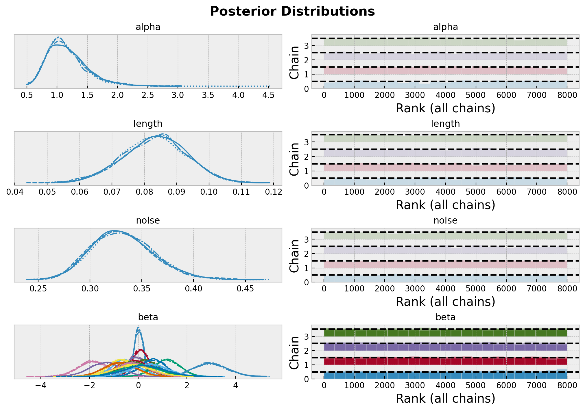
总的来说，模型似乎收敛得很好。

后验预测分布

最后，我们从测试集上的后验预测分布生成样本并绘制结果。

predictive = Predictive(model, mcmc.get_samples())
posterior_predictive = predictive(rng_subkey, x_test_centered, ell, m, non_centered)
rng_key, rng_subkey = random.split(rng_key)

idata.extend(az.from_numpyro(posterior_predictive=posterior_predictive))

fig, ax = plt.subplots()
ax.axvline(x=0, color="C2", alpha=0.8, linestyle="--", linewidth=2)
ax.axvline(
    x=1, color="C2", linestyle="--", alpha=0.8, linewidth=2, label="training range"
)
az.plot_hdi(
    x_test,
    idata.posterior_predictive["likelihood"],
    hdi_prob=0.94,
    color="C1",
    smooth=False,
    fill_kwargs={"alpha": 0.1, "label": "$94\\%$ HDI (test)"},
    ax=ax,
)
az.plot_hdi(
    x_test,
    idata.posterior_predictive["likelihood"],
    hdi_prob=0.5,
    color="C1",
    smooth=False,
    fill_kwargs={"alpha": 0.3, "label": "$50\\%$ HDI (test)"},
    ax=ax,
)
ax.plot(
    x_test,
    idata.posterior_predictive["likelihood"].mean(dim=("chain", "draw")),
    color="C1",
    linewidth=3,
    label="posterior predictive mean (test)",
)
ax.scatter(x_train, y_train_obs, c="C0", label="observed (train)")
ax.scatter(x_test, y_test_obs, c="C1", label="observed (test)")
ax.plot(x_train, y_train, color="black", linewidth=3, alpha=0.7, label="mean (latent)")
ax.legend(loc="upper center", bbox_to_anchor=(0.5, -0.1), ncol=4)
ax.set(xlabel="x", ylabel="y")
ax.set_title("Posterior Predictive", fontsize=16, fontweight="bold");

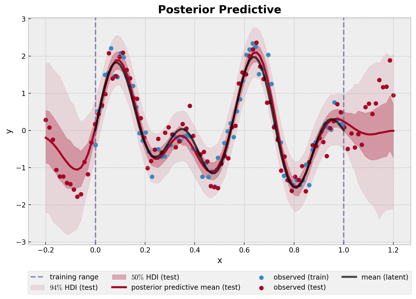
该模型很好地捕捉了训练集区域的基础函数。随着远离训练集，不确定性会增加。

---

希尔伯特空间近似的原理？

在本 notebook 中，我们不会深入探讨希尔伯特空间近似的细节。然而，这里我们概述其主要思想。

我们用一组基函数 \(\phi_{j}\) 来近似核函数，这些基函数来自区间 [-ell, ell] 中狄利克雷拉普拉斯算子的谱。这些基函数独立于核超参数 alpha 和 length！这些基函数的权重来自于在狄利克雷拉普拉斯算子的特征值 \(\lambda_{j}\) 的平方根处评估核函数的谱密度 \(S(\omega)\)。最终的近似公式如下：

\[f(x) \approx \sum_{j = 1}^{m} \overbrace{\color{red}{\left(S(\sqrt{\lambda_j})\right)^{1/2}}}^{\text{所有超参数都在这里！}} \times \underbrace{\color{blue}{\phi_{j}(x)}}_{\text{易于计算！}} \times \overbrace{\color{green}{\beta_{j}}}^{\sim \: \text{Normal}(0,1)}\]

让我们看看近似的组成部分。首先，我们绘制基函数。

basis = eigenfunctions(x=x_train_centered, ell=ell, m=m)

fig, ax = plt.subplots()
ax.plot(x_train_centered, basis)
ax.set(xlabel="x_centered")
ax.set_title("Laplacian Eigenfunctions", fontsize=16, fontweight="bold");

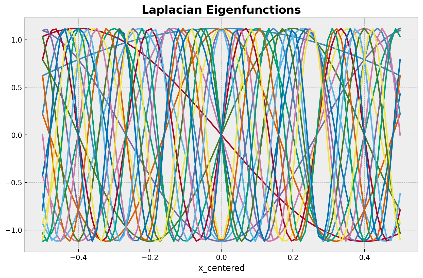
这些基函数由谱密度值加权。下面的图显示了在狄利克雷拉普拉斯算子特征值的平方根上评估的谱密度。我们使用不同的超参数值 alpha 和 length 来查看谱密度如何变化。我们还用黑色绘制了使用从上面模型推断出的后验均值对应的谱密度。

alpha_posterior_mean = idata.posterior["alpha"].mean(dim=("chain", "draw")).item()
length_posterior_mean = idata.posterior["length"].mean(dim=("chain", "draw")).item()

fig, ax = plt.subplots()
ax.set(xlabel="index eigenvalue (sorted)", ylabel="spectral density")

for alpha_value in (1.0, 1.5):
    for length_value in (0.05, 0.1):
        diag_sd = diag_spectral_density_squared_exponential(
            alpha=alpha_value,
            length=length_value,
            ell=ell,
            m=m,
            dim=1,
        )
        ax.plot(
            range(1, m + 1),
            diag_sd,
            marker="o",
            linewidth=1.5,
            markersize=4,
            alpha=0.8,
            label=f"alpha = {alpha_value}, length = {length_value}",
        )

diag_sd = diag_spectral_density_squared_exponential(
    alpha=alpha_posterior_mean,
    length=length_posterior_mean,
    ell=ell,
    m=m,
    dim=1,
)
ax.plot(
    range(1, m + 1),
    diag_sd,
    marker="o",
    color="black",
    linewidth=3,
    markersize=6,
    label=f"posterior mean (alpha = {alpha_posterior_mean: .2f}, length = {length_posterior_mean: .2f})",
)
ax.xaxis.set_major_locator(MultipleLocator())
ax.legend(loc="upper right", title="Hyperparameters")
ax.set_title(
    r"Spectral Density on the First $m$ (square root) Eigenvalues",
    fontsize=16,
    fontweight="bold",
);

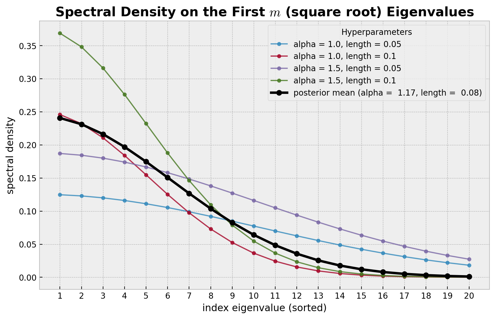
随着谱密度在高频处衰减到零，较大特征值的影响变得越来越小。可以证明，在极限情况下，希尔伯特空间近似收敛于真实的核函数。