分层预测
在本 notebook 中,我们将 Pyro 分层多元预测示例从预测 III:分层模型教程移植到 NumPyro。
我们使用 BART 列车乘客量数据集,其中包含 BART 系统中所有站点之间每小时的行程次数。我们的目标是预测未来每对站点的行程次数。我们不希望对每对站点单独进行预测,而是利用站间结构和其他特征(季节性)来生成预测。
这个模型移植最初发表在博客文章从 Pyro 到 NumPyro:分层模型预测 - 第二部分中。
准备 Notebook
[1]:
import arviz as az
import matplotlib.pyplot as plt
import numpy as np

import jax
from jax import Array, random
import jax.numpy as jnp
import optax

import numpyro
import numpyro.distributions as dist
from numpyro.examples.datasets import load_bart_od
from numpyro.infer import SVI, Predictive, Trace_ELBO
from numpyro.infer.autoguide import AutoNormal
from numpyro.infer.reparam import LocScaleReparam

plt.style.use("bmh")
plt.rcParams["figure.figsize"] = [12, 7]
plt.rcParams["figure.dpi"] = 100
plt.rcParams["figure.facecolor"] = "white"

numpyro.set_host_device_count(n=4)

rng_key = random.PRNGKey(seed=42)

assert numpyro.__version__.startswith("0.18.0")

%load_ext autoreload
%autoreload 2
%config InlineBackend.figure_format = "retina"
[2]:
!pip install -q numpyro@git+https://github.com/pyro-ppl/numpyro arviz matplotlib optax
读取数据
让我们加载数据。
[3]:
dataset = load_bart_od()
print(dataset.keys())
print(dataset["counts"].shape)
print(" ".join(dataset["stations"]))
dict_keys(['stations', 'start_date', 'counts'])
(78888, 50, 50)
12TH 16TH 19TH 24TH ANTC ASHB BALB BAYF BERY CAST CIVC COLM COLS CONC DALY DBRK DELN DUBL EMBR FRMT FTVL GLEN HAYW LAFY LAKE MCAR MLBR MLPT MONT NBRK NCON OAKL ORIN PCTR PHIL PITT PLZA POWL RICH ROCK SANL SBRN SFIA SHAY SSAN UCTY WARM WCRK WDUB WOAK
回顾一下,我们的目标是建模从所有站点到所有其他站点的所有行程。对于更简单的预测任务,您可以查看入门示例
[4]:
data = jnp.log1p(np.permute_dims(dataset["counts"], (1, 2, 0)))
T = data.shape[-2]
print(data.shape)
(50, 50, 78888)
训练集 - 测试集划分
与 Pyro 示例类似,我们进行训练集和测试集划分。
[5]:
T2 = data.shape[-1]  # end
T1 = T2 - 24 * 7 * 2  # train/test split
T0 = T1 - 24 * 90  # beginning: train on 90 days of data
[6]:
y = data[..., T0:T2]
y_train = data[..., T0:T1]
y_test = data[..., T1:T2]

print(f"y: {y.shape}")
print(f"y_train: {y_train.shape}")
print(f"y_test: {y_test.shape}")
y: (50, 50, 2496)
y_train: (50, 50, 2160)
y_test: (50, 50, 336)
[7]:
n_stations = y_train.shape[-2]

time = jnp.array(range(T0, T2))
time_train = jnp.array(range(T0, T1))
t_max_train = time_train.size

time_test = jnp.array(range(T1, T2))
t_max_test = time_test.size

covariates = jnp.zeros_like(y)
covariates_train = jnp.zeros_like(y_train)
covariates_test = jnp.zeros_like(y_test)

assert time_train.size + time_test.size == time.size
assert y_train.shape == (n_stations, n_stations, t_max_train)
assert y_test.shape == (n_stations, n_stations, t_max_test)
assert covariates.shape == y.shape
assert covariates_train.shape == y_train.shape
assert covariates_test.shape == y_test.shape
重复季节性特征
为了建模每周季节性,Pyro 提供了一个非常便利的辅助函数 periodic_repeat <https://docs.pyro.org.cn/en/stable/ops.html#pyro.ops.tensor_utils.periodic_repeat> 来重复季节性特征。这里我们提供了该函数的 JAX 版本。
[8]:
def periodic_repeat_jax(tensor: Array, size: int, dim: int) -> Array:
    """
    Repeat a period-sized tensor up to given size using JAX.

    Parameters
    ----------
    tensor : Array
        A JAX array to be repeated.
    size : int
        Desired size of the result along dimension `dim`.
    dim : int
        The tensor dimension along which to repeat.

    Returns
    -------
    Array
        The repeated tensor.

    References
    ----------
    https://docs.pyro.org.cn/en/stable/ops.html#pyro.ops.tensor_utils.periodic_repeat
    """
    assert isinstance(size, int) and size >= 0
    assert isinstance(dim, int)
    if dim >= 0:
        dim -= tensor.ndim

    period = tensor.shape[dim]
    repeats = [1] * tensor.ndim
    repeats[dim] = (size + period - 1) // period
    result = jnp.tile(tensor, repeats)

    slices = [slice(None)] * tensor.ndim
    slices[dim] = slice(None, size)

    return result[tuple(slices)]
模型设定
以下是预测模型的主要组成部分
局部水平动态受目的地站点驱动。我们使用分层结构来建模局部水平分量的所有目的地级别漂移。由于这些分层模型可能具有奇怪的采样几何,我们也从数据中学习重新参数化参数。
季节性分量和噪声尺度是出发站和目的地站的总和。
为了让一切更具体,让我们看看代码中的模型结构。
[9]:
def model(covariates: Array, y: Array | None = None) -> None:
    # Get the time and feature dimensions
    n_series, n_series, t_max = covariates.shape

    # Define the plates to be able to use them below
    origin_plate = numpyro.plate("origin", n_series, dim=-3)
    destin_plate = numpyro.plate("destin", n_series, dim=-2)
    hour_of_week_plate = numpyro.plate("hour_of_week", 24 * 7, dim=-1)

    # Global scale for the drift
    drift_scale = numpyro.sample("drift_scale", dist.LogNormal(loc=-20, scale=5))

    # Sample the centered parameter for the LocScaleReparam
    destin_centered = numpyro.sample("destin_centered", dist.Uniform(low=0, high=1))

    with origin_plate, hour_of_week_plate:
        origin_seasonal = numpyro.sample("origin_seasonal", dist.Normal(loc=0, scale=5))

    with destin_plate:
        with (
            numpyro.plate("time", t_max),
            numpyro.handlers.reparam(
                config={"drift": LocScaleReparam(centered=destin_centered)}
            ),
        ):
            # Sample the drift parameters
            # We have one drift parameter per time series (station) and time point
            drift = numpyro.sample("drift", dist.Normal(loc=0, scale=drift_scale))

        with hour_of_week_plate:
            # Sample the seasonal parameters
            # We have one seasonal parameter per hour of the week and per station
            destin_seasonal = numpyro.sample(
                "destin_seasonal", dist.Normal(loc=0, scale=5)
            )

    # We model a static pairwise station->station affinity, which e.g.
    # can compensate for the fact that people tend not to travel from
    # a station to itself.
    with origin_plate, destin_plate:
        pairwise = numpyro.sample("pairwise", dist.Normal(0, 1))

    # We model the origin and destination scales separately
    # and then add them together to get the final scale.
    with origin_plate:
        origin_scale = numpyro.sample("origin_scale", dist.LogNormal(-5, 5))
    with destin_plate:
        destin_scale = numpyro.sample("destin_scale", dist.LogNormal(-5, 5))
        scale = origin_scale + destin_scale

    # Repeat the seasonal parameters to match the length of the time series
    seasonal = origin_seasonal + destin_seasonal
    seasonal_repeat = periodic_repeat_jax(seasonal, t_max, dim=-1)

    # Define the local level transition function
    def transition_fn(carry, t):
        "Local level transition function"
        previous_level = carry
        current_level = previous_level + drift[..., t]
        return current_level, current_level

    # Compute the latent levels using scan
    _, pred_levels = jax.lax.scan(
        transition_fn, init=jnp.zeros((n_series,)), xs=jnp.arange(t_max)
    )

    # We need to transpose the prediction levels to match the shape of the data
    pred_levels = pred_levels.transpose(1, 0)

    # Compute the mean of the model
    mu = pred_levels + seasonal_repeat + pairwise

    # Sample the observations
    with numpyro.handlers.condition(data={"obs": y}):
        numpyro.sample("obs", dist.Normal(loc=mu, scale=scale))
让我们可视化模型结构。
[10]:
numpyro.render_model(
    model=model,
    model_kwargs={"covariates": covariates_train, "y": y_train},
    render_distributions=True,
    render_params=True,
)
[10]:

先验预测检验
像往常一样(强烈推荐!),我们应该执行先验预测检验。
[11]:
prior_predictive = Predictive(model=model, num_samples=500, return_sites=["obs"])

rng_key, rng_subkey = random.split(rng_key)

prior_samples = prior_predictive(rng_subkey, covariates_train)

idata_prior = az.from_dict(
    prior_predictive={k: v[None, ...] for k, v in prior_samples.items()},
    coords={
        "time_train": time_train,
        "origin": dataset["stations"],
        "destin": dataset["stations"],
    },
    dims={"obs": ["origin", "destin", "time_train"]},
)
让我们绘制目的地站点 ANTC 的前 \(8\) 个站点的先验预测分布。
[12]:
station = "ANTC"
idx = np.nonzero(dataset["stations"] == station)[0].item()

fig, axes = plt.subplots(
    nrows=8, ncols=1, figsize=(12, 15), sharex=True, sharey=True, layout="constrained"
)
for i, ax in enumerate(axes):
    for j, hdi_prob in enumerate([0.94, 0.5]):
        az.plot_hdi(
            time_train[time_train >= T1 - 3 * (24 * 7)],
            idata_prior["prior_predictive"]["obs"]
            .sel(destin=station)
            .isel(origin=i)[:, :, np.array(time_train) >= T1 - 3 * (24 * 7)]
            .clip(min=0),
            hdi_prob=hdi_prob,
            color="C0",
            fill_kwargs={
                "alpha": 0.3 + 0.2 * j,
                "label": f"{hdi_prob * 100:.0f}% HDI (train)",
            },
            smooth=False,
            ax=ax,
        )

    ax.plot(
        time_train[time_train >= T1 - 3 * (24 * 7)],
        data[i, idx, T1 - 3 * (24 * 7) : T1],
        "black",
        lw=1,
        label="Truth",
    )

    ax.legend(
        bbox_to_anchor=(1.05, 1), loc="upper left", borderaxespad=0.0, fontsize=12
    )

fig.suptitle("Prior predictive checks", fontsize=18, fontweight="bold");
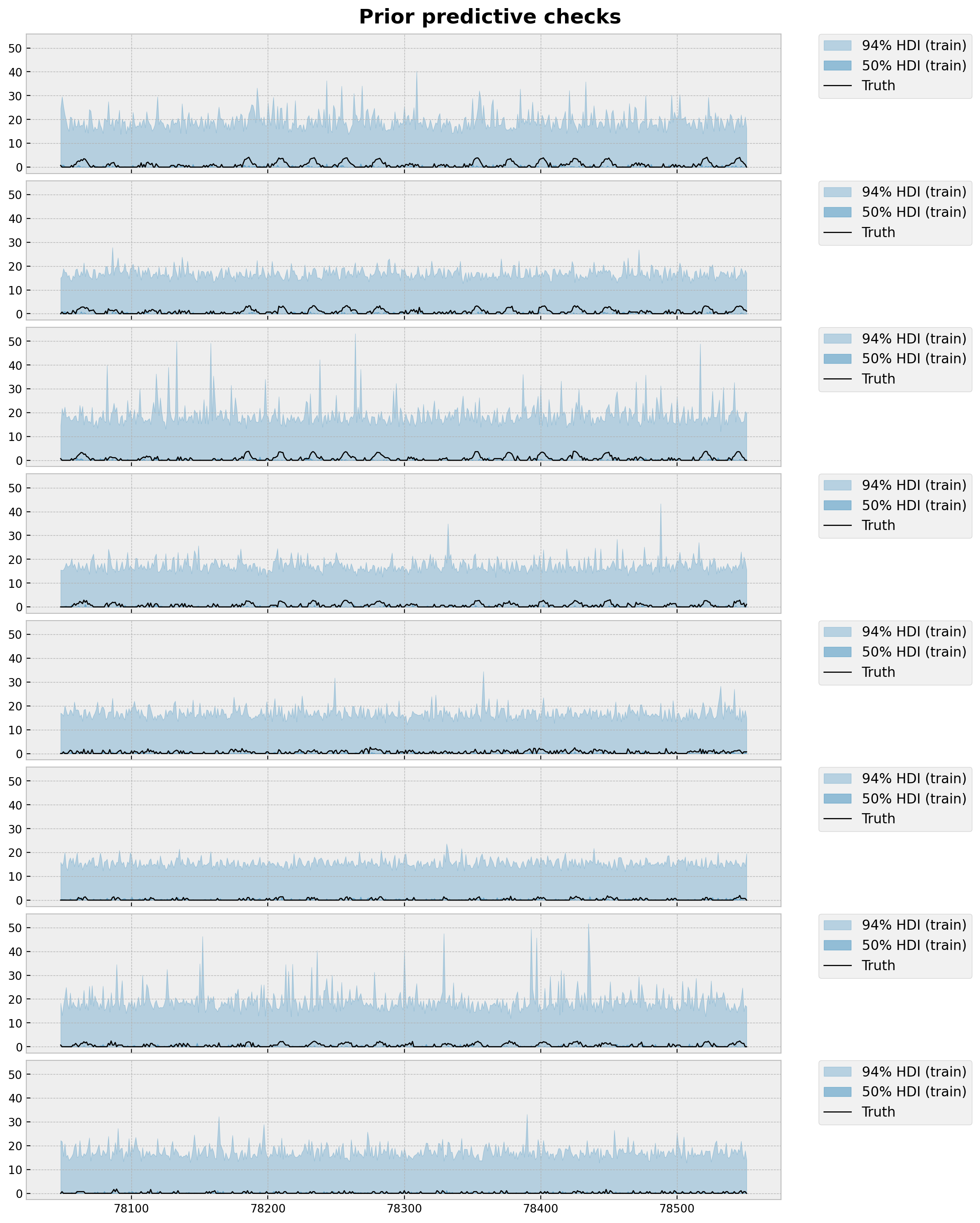
总的来说,先验范围看起来非常合理。
使用 SVI 进行推断
现在我们使用随机变分推断将模型拟合到数据。
[13]:
%%time

# See https://optax.readthedocs.io/en/stable/getting_started.html#custom-optimizers
scheduler = optax.linear_onecycle_schedule(
    transition_steps=8_000,
    peak_value=0.1,
    pct_start=0.1,
    pct_final=0.7,
    div_factor=2,
    final_div_factor=4,
)

optimizer = optax.chain(
    optax.clip_by_global_norm(1.0),
    optax.scale_by_adam(),
    optax.scale_by_schedule(scheduler),
    optax.scale(-1.0),
)


guide = AutoNormal(model)
optimizer = optimizer
svi = SVI(model, guide, optimizer, loss=Trace_ELBO())
num_steps = 8_000

rng_key, rng_subkey = random.split(key=rng_key)

svi_result = svi.run(rng_subkey, num_steps, covariates_train, y_train)

fig, ax = plt.subplots(figsize=(9, 6))
ax.plot(svi_result.losses)
ax.set_yscale("log")
ax.set_title("ELBO loss", fontsize=18, fontweight="bold");
100%|██████████| 8000/8000 [02:54<00:00, 45.80it/s, init loss: 8788430848.0000, avg. loss [7601-8000]: 3667545.0000]
CPU times: user 8min 51s, sys: 1min 17s, total: 10min 8s
Wall time: 3min 2s
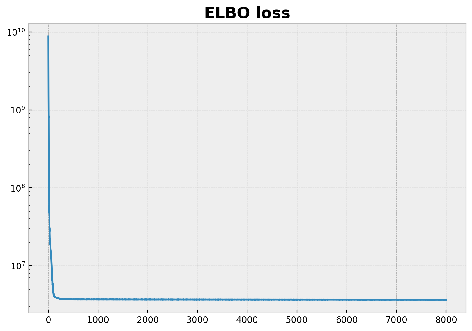
得到的 ELBO 损失不错!
后验预测检验
接下来,我们为每对站点的预测生成后验预测样本。
[14]:
posterior = Predictive(
    model=model,
    guide=guide,
    params=svi_result.params,
    num_samples=200,
    return_sites=["obs"],
)
[15]:
rng_key, rng_subkey = random.split(rng_key)

idata_train = az.from_dict(
    posterior_predictive={
        k: v[None, ...] for k, v in posterior(rng_subkey, covariates_train).items()
    },
    coords={
        "time_train": time_train,
        "origin": dataset["stations"],
        "destin": dataset["stations"],
    },
    dims={"obs": ["origin", "destin", "time_train"]},
)

idata_test = az.from_dict(
    posterior_predictive={
        k: v[None, ...] for k, v in posterior(rng_subkey, covariates).items()
    },
    coords={
        "time": time,
        "origin": dataset["stations"],
        "destin": dataset["stations"],
    },
    dims={"obs": ["origin", "destin", "time"]},
)
模型评估
为了评估模型性能,我们计算训练集和测试集的 CRPS。我们还将用于计算(经验)CRPS 的 Pyro 代码(见此处)移植到 JAX。
为了比较,我们截断数据以确保预测结果非负。
[16]:
def crps(truth: Array, pred: Array) -> float:
    """Compute the CRPS for a given truth and prediction.

    Parameters
    ----------
    truth : Array
        The truth values.
    pred : Array
        A set of sample predictions batched on rightmost dim.
        This should have shape ``(num_samples,) + truth.shape``

    Returns
    -------
    crps : float
        The average CRPS score.

    References
    ----------
    https://docs.pyro.org.cn/en/stable/_modules/pyro/ops/stats.html
    """
    if pred.shape[1:] != (1,) * (pred.ndim - truth.ndim - 1) + truth.shape:
        raise ValueError(
            f"""Expected pred to have one extra sample dim on left.
            Actual shapes: {pred.shape} versus {truth.shape}"""
        )

    absolute_error = jnp.mean(jnp.abs(pred - truth), axis=0)

    num_samples = pred.shape[0]
    if num_samples == 1:
        return jnp.average(absolute_error)

    pred = jnp.sort(pred, axis=0)
    diff = pred[1:] - pred[:-1]
    weight = jnp.arange(1, num_samples) * jnp.arange(num_samples - 1, 0, -1)
    weight = weight.reshape(weight.shape + (1,) * (diff.ndim - 1))

    per_obs_crps = absolute_error - jnp.sum(diff * weight, axis=0) / num_samples**2
    return jnp.average(per_obs_crps)


crps_train = crps(
    y_train,
    jnp.array(idata_train["posterior_predictive"]["obs"].sel(chain=0).clip(min=0)),
)

crps_test = crps(
    y_test,
    jnp.array(
        idata_test["posterior_predictive"]["obs"]
        .sel(chain=0)
        .sel(time=slice(T1, T2))
        .clip(min=0)
    ),
)
最后,我们重现了 Pyro 示例中的模型拟合和图。
[17]:
station = "ANTC"
idx = np.nonzero(dataset["stations"] == station)[0].item()

fig, axes = plt.subplots(
    nrows=8, ncols=1, figsize=(12, 15), sharex=True, sharey=True, layout="constrained"
)
for i, ax in enumerate(axes):
    for j, hdi_prob in enumerate([0.94, 0.5]):
        az.plot_hdi(
            time_train[time_train >= T1 - 24 * 7],
            idata_train["posterior_predictive"]["obs"]
            .sel(destin=station)
            .isel(origin=i)[:, :, np.array(time_train) >= T1 - 24 * 7]
            .clip(min=0),
            hdi_prob=hdi_prob,
            color="C0",
            fill_kwargs={
                "alpha": 0.3 + 0.2 * j,
                "label": f"{hdi_prob * 100:.0f}% HDI (train)",
            },
            smooth=False,
            ax=ax,
        )

        az.plot_hdi(
            time[time >= T1],
            idata_test["posterior_predictive"]["obs"]
            .sel(destin=station)
            .isel(origin=i)[:, :, np.array(time) >= T1]
            .clip(min=0),
            hdi_prob=hdi_prob,
            color="C1",
            fill_kwargs={
                "alpha": 0.2 + 0.2 * j,
                "label": f"{hdi_prob * 100:.0f}% HDI (test)",
            },
            smooth=False,
            ax=ax,
        )

    christmas_index = 78736
    ax.axvline(christmas_index, color="C2", lw=20, alpha=0.2, label="Christmas")

    ax.plot(
        time[time >= T1 - 24 * 7],
        data[i, idx, T1 - 24 * 7 : T2],
        "black",
        lw=1,
        label="Truth",
    )

    ax.axvline(T1, color="C3", linestyle="--", label="Train/test split")

    ax.legend(
        bbox_to_anchor=(1.05, 1),
        loc="upper left",
        borderaxespad=0.0,
        fontsize=9,
        labelspacing=0.6,
    )

fig.suptitle(
    f"""Posterior predictive checks

    Train CRPS: {crps_train:.4f} | Test CRPS: {crps_test:.4f}
    """,
    fontsize=18,
    fontweight="bold",
);
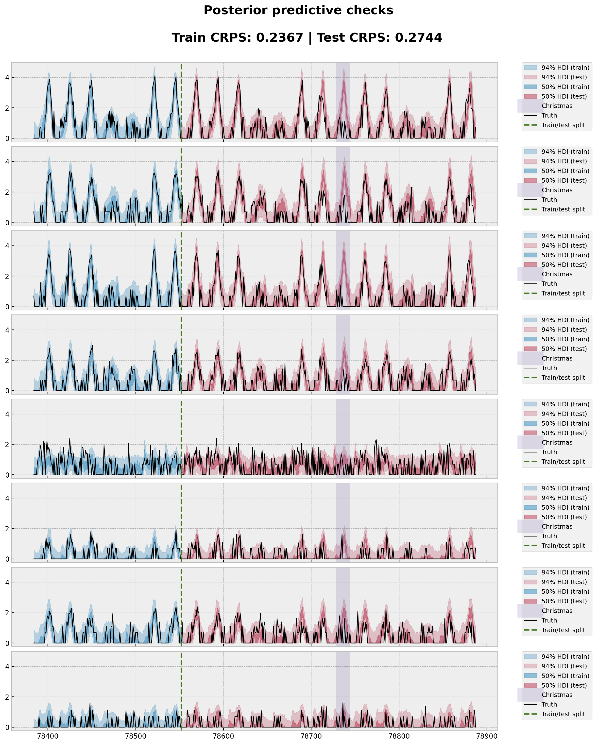
总的来说,预测看起来相当不错!