交互式在线版本：

NNX 和 NumPyro 集成

在此示例 notebook 中，我们将展示如何将来自 NNX 库的神经网络组件集成到 NumPyro 模型中。以类似的方式，您也可以使用 Flax Linen API。

此 notebook 基于博客文章 Flax and NumPyro Toy Example。

准备 Notebook

!pip install -q numpyro@git+https://github.com/pyro-ppl/numpyro arviz flax matplotlib

import arviz as az
import matplotlib.pyplot as plt
import numpy as np

from flax import nnx
from jax import random
import jax.numpy as jnp

import numpyro
from numpyro.contrib.module import nnx_module, random_nnx_module
import numpyro.distributions as dist
from numpyro.handlers import condition
from numpyro.infer import SVI, Trace_ELBO
from numpyro.infer.autoguide import AutoNormal
from numpyro.infer.util import Predictive

plt.style.use("bmh")
plt.rcParams["figure.figsize"] = [10, 6]
plt.rcParams["figure.dpi"] = 100
plt.rcParams["figure.facecolor"] = "white"

numpyro.set_host_device_count(n=4)

rng_key = random.PRNGKey(seed=42)

%load_ext autoreload
%autoreload 2
%config InlineBackend.figure_format = "retina"

生成数据

我们生成了一个均值和标准差均非线性的合成数据集。

n = 32 * 10
rng_key, rng_subkey = random.split(rng_key)
x = jnp.linspace(1, jnp.pi, n)
mu_true = jnp.sqrt(x + 0.5) * jnp.sin(9 * x)
sigma_true = 0.15 * x**2
rng_key, rng_subkey = random.split(rng_key)
y = mu_true + sigma_true * random.normal(rng_key, shape=(n,))

让我们可视化生成的数据集

fig, ax = plt.subplots()
ax.plot(x, mu_true, color="C0", label=r"$\mu$", linewidth=3)
ax.fill_between(
    x,
    (mu_true - 2 * sigma_true),
    (mu_true + 2 * sigma_true),
    color="C0",
    alpha=0.2,
    label=r"$\mu \pm 2 \sigma$",
)
ax.scatter(x, y, color="black", label="data")
ax.legend(loc="upper left")
ax.set_title(label="Simulated Data", fontsize=18, fontweight="bold")
ax.set(xlabel="x", ylabel="y");

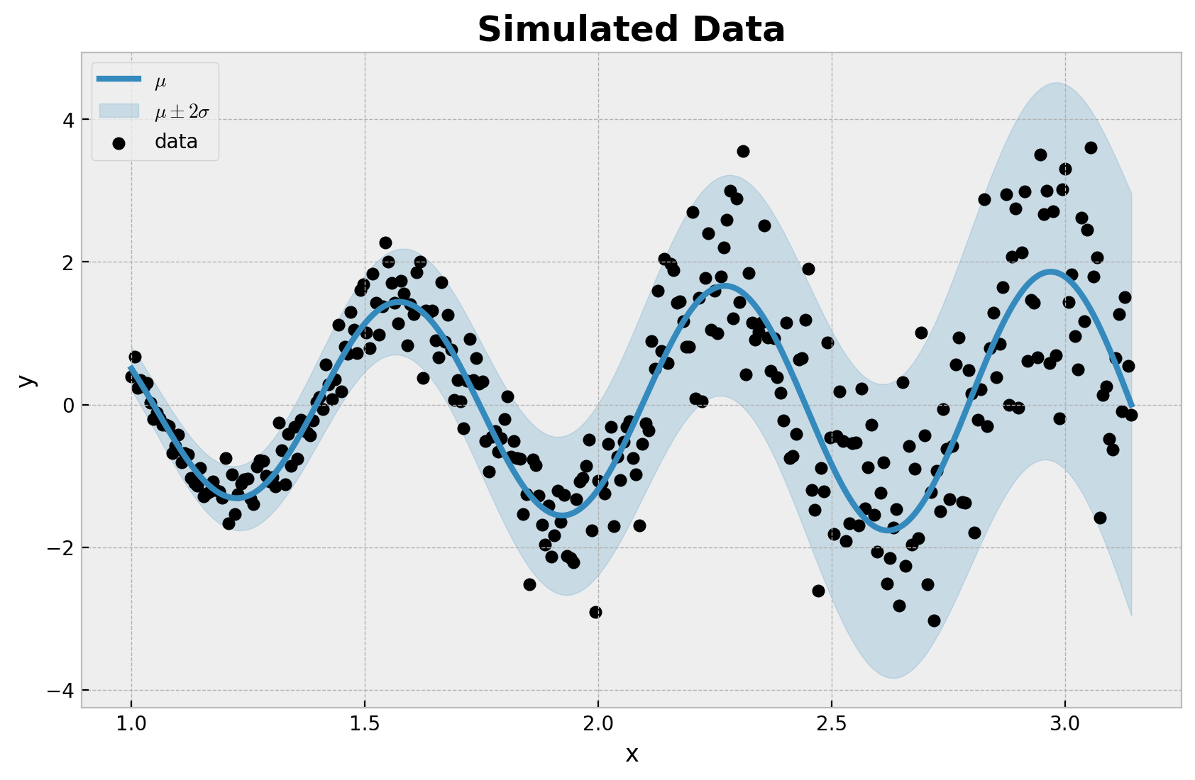
我们清楚地看到数据是非线性的，并且存在异方差噪声。我们希望使用神经网络对非线性进行建模，将数据的均值和标准差建模为输入 \(x\) 的函数。

模型规范

首先，我们准备训练数据。

x_train = x[..., None]
y_train = y

接下来，我们使用 NNX 定义两个 MLP 组件，一个用于均值，一个用于标准差。您可以查看 `NNX basics <https://flax.org.cn/en/v0.8.3/experimental/nnx/nnx_basics.html>`__ 以获取更多详细信息。

class LocMLP(nnx.Module):
    """3-layer Multi-layer perceptron for the mean."""

    def __init__(self, din: int, dmid: int, dout: int, *, rngs: nnx.Rngs):
        self.linear1 = nnx.Linear(din, dmid, rngs=rngs)
        self.linear2 = nnx.Linear(dmid, dmid, rngs=rngs)
        self.linear3 = nnx.Linear(dmid, dout, rngs=rngs)

    def __call__(self, x, rngs=None):
        x = self.linear1(x)
        x = nnx.sigmoid(x)
        x = self.linear2(x)
        x = nnx.sigmoid(x)
        x = self.linear3(x)
        return x


class ScaleMLP(nnx.Module):
    """Single-layer MLP for the standard deviation."""

    def __init__(self, *, rngs: nnx.Rngs) -> None:
        self.linear = nnx.Linear(1, 1, rngs=rngs)

    def __call__(self, x, rngs=None):
        x = self.linear(x)
        return nnx.softplus(x)

现在我们以“即时”（eager）方式定义神经网络组件。

mu_nn_module = LocMLP(din=1, dmid=8, dout=1, rngs=nnx.Rngs(0))

sigma_nn_module = ScaleMLP(rngs=nnx.Rngs(1))

最后，我们可以将神经网络组件添加到 NumPyro 模型中，我们在其中使用正态分布作为似然函数，并允许参数随输入 \(x\) 变化。

def model(x):
    # Neural network component for the mean. Here we consider the parameters of the
    # neural network as learnable.
    mu_nn = nnx_module("mu_nn", mu_nn_module)
    # Here we consider the parameters of the neural network as random variables.
    # Hence we can set priors for them.
    sigma_nn = random_nnx_module(
        "sigma_nn",
        sigma_nn_module,
        prior={
            # From the data we know the variance is increasing over x.
            # Hence we use a HalfNormal distribution to model the kernel term.
            "linear.kernel": dist.HalfNormal(scale=1),
            # We use a Normal distribution for the bias.
            "linear.bias": dist.Normal(loc=0, scale=1),
        },
    )

    mu = numpyro.deterministic("mu", mu_nn(x).squeeze())

    sigma = numpyro.deterministic("sigma", sigma_nn(x).squeeze())

    with numpyro.plate("data", len(x)):
        numpyro.sample("likelihood", dist.Normal(loc=mu, scale=sigma))


numpyro.render_model(
    model=model,
    model_args=(x_train,),
    render_distributions=True,
    render_params=True,
)

先验预测检查

在进行推断之前，我们可以检查先验预测分布，以确保先验是合理的。

prior_predictive = Predictive(model=model, num_samples=100)
rng_key, rng_subkey = random.split(key=rng_key)
prior_predictive_samples = prior_predictive(rng_subkey, x_train)

obs_train = jnp.arange(x_train.size)

idata = az.from_dict(
    prior_predictive={
        k: np.expand_dims(a=np.asarray(v), axis=0)
        for k, v in prior_predictive_samples.items()
    },
    coords={"obs": obs_train},
    dims={"mu": ["obs"], "sigma": ["obs"], "likelihood": ["obs"]},
)

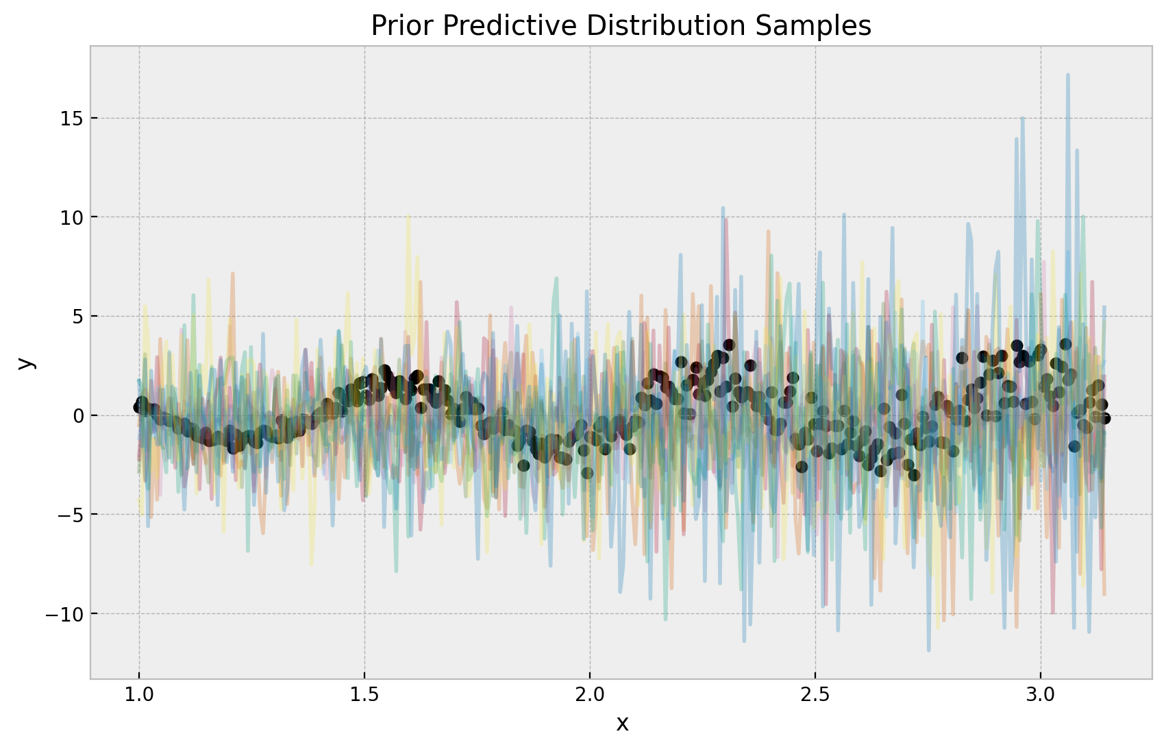
首先，我们可视化先验预测分布。我们清楚地看到方差随着 \(x\) 的增加而增加，正如我们预期的那样（由先验定义）。我们也看到样本的范围与数据在一个合理的范围内。

fig, ax = plt.subplots()

for i in range(10):
    ax.plot(x, idata["prior_predictive"]["likelihood"].sel(chain=0, draw=i), alpha=0.25)
ax.scatter(x, y, color="black", label="data")
ax.set(xlabel="x", ylabel="y", title="Prior Predictive Distribution Samples");

我们还可以验证 sigma 核的先验是否按预期工作

fig, ax = plt.subplots()

az.plot_dist(
    idata["prior_predictive"]["sigma_nn/linear.kernel"].squeeze(axis=(-1, -2)),
    color="C2",
    fill_kwargs={"alpha": 0.3},
)

ax.set(
    xlabel="sigma_nn/linear.kernel",
    title="Prior Predictive Distribution - Kernel of the Standard Deviation MLP",
);

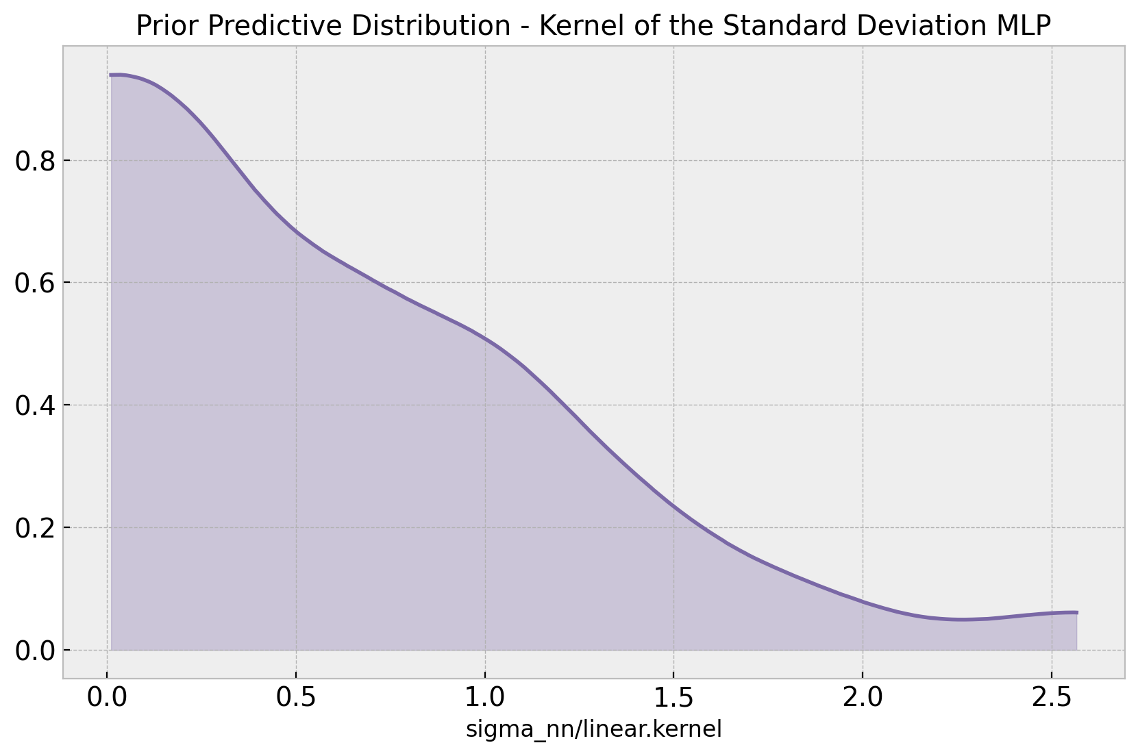
我们确实看到先验是正的！

模型推断

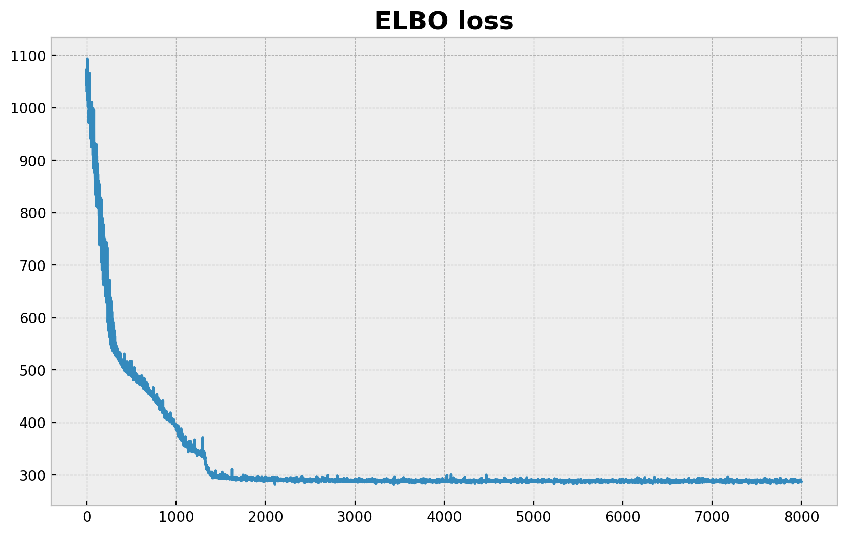
现在我们使用 SVI 对模型进行推断。

# We condition the model on the training data
conditioned_model = condition(model, data={"likelihood": y_train})

guide = AutoNormal(model=conditioned_model)
optimizer = numpyro.optim.Adam(step_size=0.005)
svi = SVI(conditioned_model, guide, optimizer, loss=Trace_ELBO())
n_samples = 8_000
rng_key, rng_subkey = random.split(key=rng_key)
svi_result = svi.run(rng_subkey, n_samples, x_train)

fig, ax = plt.subplots()
ax.plot(svi_result.losses)
ax.set_title("ELBO loss", fontsize=18, fontweight="bold");

100%|██████████| 8000/8000 [00:01<00:00, 5976.75it/s, init loss: 1032.5969, avg. loss [7601-8000]: 287.5595]

现在我们生成后验预测分布。

params = svi_result.params
posterior_predictive = Predictive(
    model=model,
    guide=guide,
    params=params,
    num_samples=2_000,
    return_sites=["mu", "sigma", "likelihood"],
)
rng_key, rng_subkey = random.split(key=rng_key)
posterior_predictive_samples = posterior_predictive(rng_subkey, x_train)

现在我们收集后验预测样本以便进行可视化。

idata.extend(
    az.from_dict(
        posterior_predictive={
            k: np.expand_dims(a=np.asarray(v), axis=0)
            for k, v in posterior_predictive_samples.items()
        },
        coords={"obs": obs_train},
        dims={"mu": ["obs"], "sigma": ["obs"], "likelihood": ["obs"]},
    )
)

最后，我们可视化后验预测分布、均值和标准差组件。

fig, ax = plt.subplots(
    nrows=3,
    ncols=1,
    sharex=True,
    sharey=True,
    figsize=(10, 9),
    layout="constrained",
)

az.plot_hdi(
    x,
    idata["posterior_predictive"]["likelihood"],
    color="C1",
    fill_kwargs={"alpha": 0.3, "label": "94% HDI"},
    ax=ax[0],
)
ax[0].plot(
    x_train,
    idata["posterior_predictive"]["likelihood"].mean(dim=("chain", "draw")),
    color="C1",
    linewidth=3,
    label="SVI Posterior Mean",
)
ax[0].plot(x, mu_true, color="C0", label=r"$\mu$", linewidth=3)
ax[0].scatter(x, y, color="black", label="data")
ax[0].legend(loc="upper left")
ax[0].set(ylabel="y")
ax[0].set_title(label="Posterior Predictive Distribution")

ax[1].plot(
    x,
    idata["posterior_predictive"]["mu"].mean(dim=("chain", "draw")),
    linewidth=3,
    color="C2",
)
ax[1].set_title(label="Mean")

ax[2].plot(
    x,
    idata["posterior_predictive"]["sigma"].mean(dim=("chain", "draw")),
    linewidth=3,
    color="C3",
)
ax[2].set(xlabel="x")
ax[2].set_title(label="Standard Deviation");

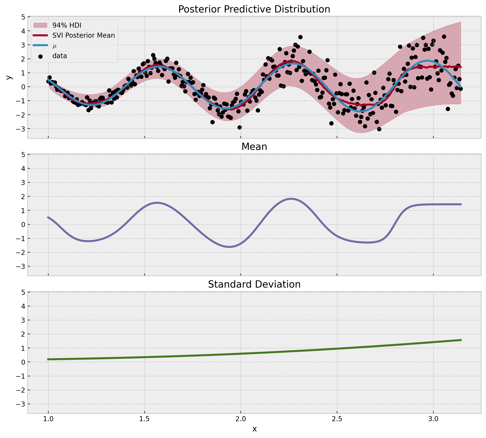
结果看起来很棒！拟合和组件都按预期工作。