注意
跳转至末尾以下载完整示例代码。
示例:高斯过程的希尔伯特空间近似。
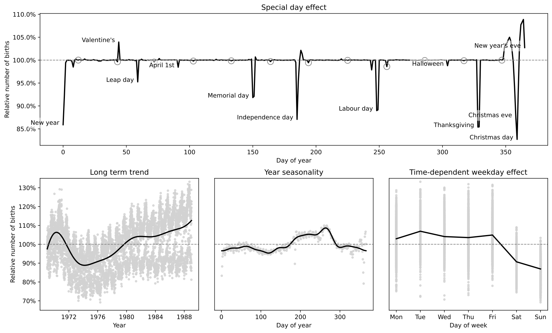
本示例重现了 Aki Vehtari [1] 的优秀案例研究(最初使用 R 和 Stan 编写)中的模型。该案例研究使用近似高斯过程 [2] 对 1969 年至 1988 年美国每天的相对出生人数进行建模。希尔伯特空间近似比精确高斯过程快得多,因为它避免了协方差矩阵求逆的需求。
原始案例研究还强调了构建贝叶斯模型的迭代过程,这对于教学资源来说非常出色。然而,在此我们只重现包含所有组件(长期趋势、平滑的年度季节性、缓慢变化的星期效应、一年中的某一天效应以及特殊浮动日效应)的模型。
模型的不同组件被隔离到单独的函数中,以便它们可以在不同的上下文中轻松重用。为了将多个组件组合成一个生日模型,我们在此使用了 Numpyro 的 scope 处理器,它通过给组件的站点名称添加前缀来修改它们。通过这样做,我们避免了模型中站点名称的重复。遵循这种模式,使用此处提供的代码可以轻松构建 [1] 中的其他模型。
我们的模型在数学细节上有一些微小的差异,这些差异是我们为了使链条充分混合或便于实现而必须进行的。我们已经对模型不同的地方进行了注释。
周期核近似需要 jax 后端的 tensorflow-probability。有关安装说明,请参阅 <https://tensorflowcn.cn/probability/examples/TensorFlow_Probability_on_JAX>。
- 参考文献
Gelman, Vehtari, Simpson 等人 (2020),“贝叶斯工作流书籍 - 生日” <https://avehtari.github.io/casestudies/Birthdays/birthdays.html>。
Riutort-Mayol G, Bürkner PC, Andersen MR 等人 (2020),“用于概率编程的实用希尔伯特空间近似贝叶斯高斯过程”。
import argparse
import os

import matplotlib.pyplot as plt
import pandas as pd

import jax
import jax.numpy as jnp
from tensorflow_probability.substrates import jax as tfp

import numpyro
from numpyro import deterministic, plate, sample
import numpyro.distributions as dist
from numpyro.handlers import scope
from numpyro.infer import MCMC, NUTS, init_to_median


# --- Data processing functions
def get_labour_days(dates):
    """
    First monday of September
    """
    is_september = dates.dt.month.eq(9)
    is_monday = dates.dt.weekday.eq(0)
    is_first_week = dates.dt.day.le(7)

    is_labour_day = is_september & is_monday & is_first_week
    is_day_after = is_labour_day.shift(fill_value=False)

    return is_labour_day | is_day_after


def get_memorial_days(dates):
    """
    Last monday of May
    """
    is_may = dates.dt.month.eq(5)
    is_monday = dates.dt.weekday.eq(0)
    is_last_week = dates.dt.day.ge(25)

    is_memorial_day = is_may & is_monday & is_last_week
    is_day_after = is_memorial_day.shift(fill_value=False)

    return is_memorial_day | is_day_after


def get_thanksgiving_days(dates):
    """
    Third thursday of November
    """
    is_november = dates.dt.month.eq(11)
    is_thursday = dates.dt.weekday.eq(3)
    is_third_week = dates.dt.day.between(22, 28)

    is_thanksgiving = is_november & is_thursday & is_third_week
    is_day_after = is_thanksgiving.shift(fill_value=False)

    return is_thanksgiving | is_day_after


def get_floating_days_indicators(dates):
    def encode(x):
        return jnp.array(x.values, dtype=jnp.result_type(int))

    return {
        "labour_days_indicator": encode(get_labour_days(dates)),
        "memorial_days_indicator": encode(get_memorial_days(dates)),
        "thanksgiving_days_indicator": encode(get_thanksgiving_days(dates)),
    }


def load_data():
    URL = "https://raw.githubusercontent.com/avehtari/casestudies/master/Birthdays/data/births_usa_1969.csv"
    data = pd.read_csv(URL, sep=",")
    day0 = pd.to_datetime("31-Dec-1968")
    dates = [day0 + pd.Timedelta(f"{i}d") for i in data["id"]]
    data["date"] = dates
    data["births_relative"] = data["births"] / data["births"].mean()
    return data


def make_birthdays_data_dict(data):
    x = data["id"].values
    y = data["births_relative"].values
    dates = data["date"]

    xsd = jnp.array((x - x.mean()) / x.std())
    ysd = jnp.array((y - y.mean()) / y.std())
    day_of_week = jnp.array((data["day_of_week"] - 1).values)
    day_of_year = jnp.array((data["day_of_year"] - 1).values)
    floating_days = get_floating_days_indicators(dates)
    period = 365.25
    w0 = x.std() * (jnp.pi * 2 / period)
    L = 1.5 * max(xsd)
    M1 = 10
    M2 = 10  # 20 in original case study
    M3 = 5

    return {
        "x": xsd,
        "day_of_week": day_of_week,
        "day_of_year": day_of_year,
        "w0": w0,
        "L": L,
        "M1": M1,
        "M2": M2,
        "M3": M3,
        **floating_days,
        "y": ysd,
    }


# --- Modelling utility functions --- #
def spectral_density(w, alpha, length):
    c = alpha * jnp.sqrt(2 * jnp.pi) * length
    e = jnp.exp(-0.5 * (length**2) * (w**2))
    return c * e


def diag_spectral_density(alpha, length, L, M):
    sqrt_eigenvalues = jnp.arange(1, 1 + M) * jnp.pi / 2 / L
    return spectral_density(sqrt_eigenvalues, alpha, length)


def eigenfunctions(x, L, M):
    """
    The first `M` eigenfunctions of the laplacian operator in `[-L, L]`
    evaluated at `x`. These are used for the approximation of the
    squared exponential kernel.
    """
    m1 = (jnp.pi / (2 * L)) * jnp.tile(L + x[:, None], M)
    m2 = jnp.diag(jnp.linspace(1, M, num=M))
    num = jnp.sin(m1 @ m2)
    den = jnp.sqrt(L)
    return num / den


def modified_bessel_first_kind(v, z):
    v = jnp.asarray(v, dtype=float)
    return jnp.exp(jnp.abs(z)) * tfp.math.bessel_ive(v, z)


def diag_spectral_density_periodic(alpha, length, M):
    """
    Not actually a spectral density but these are used in the same
    way. These are simply the first `M` coefficients of the low rank
    approximation for the periodic kernel.
    """
    a = length ** (-2)
    J = jnp.arange(0, M)
    c = jnp.where(J > 0, 2, 1)
    q2 = (c * alpha**2 / jnp.exp(a)) * modified_bessel_first_kind(J, a)
    return q2


def eigenfunctions_periodic(x, w0, M):
    """
    Basis functions for the approximation of the periodic kernel.
    """
    m1 = jnp.tile(w0 * x[:, None], M)
    m2 = jnp.diag(jnp.arange(M, dtype=jnp.float32))
    mw0x = m1 @ m2
    cosines = jnp.cos(mw0x)
    sines = jnp.sin(mw0x)
    return cosines, sines


# --- Approximate Gaussian processes --- #
def approx_se_ncp(x, alpha, length, L, M):
    """
    Hilbert space approximation for the squared
    exponential kernel in the non-centered parametrisation.
    """
    phi = eigenfunctions(x, L, M)
    spd = jnp.sqrt(diag_spectral_density(alpha, length, L, M))
    with plate("basis", M):
        beta = sample("beta", dist.Normal(0, 1))

    f = deterministic("f", phi @ (spd * beta))
    return f


def approx_periodic_gp_ncp(x, alpha, length, w0, M):
    """
    Low rank approximation for the periodic squared
    exponential kernel in the non-centered parametrisation.
    """
    q2 = diag_spectral_density_periodic(alpha, length, M)
    cosines, sines = eigenfunctions_periodic(x, w0, M)

    with plate("cos_basis", M):
        beta_cos = sample("beta_cos", dist.Normal(0, 1))

    with plate("sin_basis", M - 1):
        beta_sin = sample("beta_sin", dist.Normal(0, 1))

    # The first eigenfunction for the sine component
    # is zero, so the first parameter wouldn't contribute to the approximation.
    # We set it to zero to identify the model and avoid divergences.
    zero = jnp.array([0.0])
    beta_sin = jnp.concatenate((zero, beta_sin))

    f = deterministic("f", cosines @ (q2 * beta_cos) + sines @ (q2 * beta_sin))
    return f


# --- Components of the Birthdays model --- #
def trend_gp(x, L, M):
    alpha = sample("alpha", dist.HalfNormal(1.0))
    length = sample("length", dist.InverseGamma(10.0, 2.0))
    f = approx_se_ncp(x, alpha, length, L, M)
    return f


def year_gp(x, w0, M):
    alpha = sample("alpha", dist.HalfNormal(1.0))
    length = sample("length", dist.HalfNormal(0.2))  # scale=0.1 in original
    f = approx_periodic_gp_ncp(x, alpha, length, w0, M)
    return f


def weekday_effect(day_of_week):
    with plate("plate_day_of_week", 6):
        weekday = sample("_beta", dist.Normal(0, 1))

    monday = jnp.array([-jnp.sum(weekday)])  # Monday = 0 in original
    beta = deterministic("beta", jnp.concatenate((monday, weekday)))
    return beta[day_of_week]


def yearday_effect(day_of_year):
    slab_df = 50  # 100 in original case study
    slab_scale = 2
    scale_global = 0.1
    tau = sample(
        "tau", dist.HalfNormal(2 * scale_global)
    )  # Original uses half-t with 100df
    c_aux = sample("c_aux", dist.InverseGamma(0.5 * slab_df, 0.5 * slab_df))
    c = slab_scale * jnp.sqrt(c_aux)

    # Jan 1st:  Day 0
    # Feb 29th: Day 59
    # Dec 31st: Day 365
    with plate("plate_day_of_year", 366):
        lam = sample("lam", dist.HalfCauchy(scale=1))
        lam_tilde = jnp.sqrt(c) * lam / jnp.sqrt(c + (tau * lam) ** 2)
        beta = sample("beta", dist.Normal(loc=0, scale=tau * lam_tilde))

    return beta[day_of_year]


def special_effect(indicator):
    beta = sample("beta", dist.Normal(0, 1))
    return beta * indicator


# --- Model --- #
def birthdays_model(
    x,
    day_of_week,
    day_of_year,
    memorial_days_indicator,
    labour_days_indicator,
    thanksgiving_days_indicator,
    w0,
    L,
    M1,
    M2,
    M3,
    y=None,
):
    intercept = sample("intercept", dist.Normal(0, 1))
    f1 = scope(trend_gp, "trend")(x, L, M1)
    f2 = scope(year_gp, "year")(x, w0, M2)
    g3 = scope(trend_gp, "week-trend")(
        x, L, M3
    )  # length ~ lognormal(-1, 1) in original
    weekday = scope(weekday_effect, "week")(day_of_week)
    yearday = scope(yearday_effect, "day")(day_of_year)

    # # --- special days
    memorial = scope(special_effect, "memorial")(memorial_days_indicator)
    labour = scope(special_effect, "labour")(labour_days_indicator)
    thanksgiving = scope(special_effect, "thanksgiving")(thanksgiving_days_indicator)

    day = yearday + memorial + labour + thanksgiving
    # --- Combine components
    f = deterministic("f", intercept + f1 + f2 + jnp.exp(g3) * weekday + day)
    sigma = sample("sigma", dist.HalfNormal(0.5))
    with plate("obs", x.shape[0]):
        sample("y", dist.Normal(f, sigma), obs=y)


# --- plotting function --- #
DATA_STYLE = dict(marker=".", alpha=0.8, lw=0, label="data", c="lightgray")
MODEL_STYLE = dict(lw=2, color="k")


def plot_trend(data, samples, ax=None):
    y = data["births_relative"]
    x = data["date"]
    fsd = samples["intercept"][:, None] + samples["trend/f"]
    f = jnp.quantile(fsd * y.std() + y.mean(), 0.50, axis=0)

    if ax is None:
        ax = plt.gca()

    ax.plot(x, y, **DATA_STYLE)
    ax.plot(x, f, **MODEL_STYLE)
    return ax


def plot_seasonality(data, samples, ax=None):
    y = data["births_relative"]
    sdev = y.std()
    mean = y.mean()
    baseline = (samples["intercept"][:, None] + samples["trend/f"]) * sdev
    y_detrended = y - baseline.mean(0)
    y_year_mean = y_detrended.groupby(data["day_of_year"]).mean()
    x = y_year_mean.index

    f_median = (
        pd.DataFrame(samples["year/f"] * sdev + mean, columns=data["day_of_year"])
        .melt(var_name="day_of_year")
        .groupby("day_of_year")["value"]
        .median()
    )

    if ax is None:
        ax = plt.gca()

    ax.plot(x, y_year_mean, **DATA_STYLE)
    ax.plot(x, f_median, **MODEL_STYLE)
    return ax


def plot_week(data, samples, ax=None):
    if ax is None:
        ax = plt.gca()

    weekdays = ["Mon", "Tue", "Wed", "Thu", "Fri", "Sat", "Sun"]
    y = data["births_relative"]
    x = data["day_of_week"] - 1
    f = jnp.median(samples["week/beta"] * y.std() + y.mean(), 0)

    ax.plot(x, y, **DATA_STYLE)
    ax.plot(range(7), f, **MODEL_STYLE)
    ax.set_xticks(range(7))
    ax.set_xticklabels(weekdays)
    return ax


def plot_weektrend(data, samples, ax=None):
    dates = data["date"]
    weekdays = ["Mon", "Tue", "Wed", "Thu", "Fri", "Sat", "Sun"]
    y = data["births_relative"]
    mean, sdev = y.mean(), y.std()
    intercept = samples["intercept"][:, None]
    f1 = samples["trend/f"]
    f2 = samples["year/f"]
    g3 = samples["week-trend/f"]
    baseline = ((intercept + f1 + f2) * y.std()).mean(0)

    if ax is None:
        ax = plt.gca()

    ax.plot(dates, y - baseline, **DATA_STYLE)
    for n, day in enumerate(weekdays):
        week_beta = samples["week/beta"][:, n][:, None]
        fsd = jnp.exp(g3) * week_beta
        f = jnp.quantile(fsd * sdev + mean, 0.50, axis=0)
        ax.plot(dates, f, **MODEL_STYLE)
        ax.text(dates.iloc[-1], f[-1], day)

    return ax


def plot_1988(data, samples, ax=None):
    indicators = get_floating_days_indicators(data["date"])
    memorial_beta = samples["memorial/beta"][:, None]
    labour_beta = samples["labour/beta"][:, None]
    thanks_beta = samples["thanksgiving/beta"][:, None]

    memorials = indicators["memorial_days_indicator"] * memorial_beta
    labour = indicators["labour_days_indicator"] * labour_beta
    thanksgiving = indicators["thanksgiving_days_indicator"] * thanks_beta
    floating_days = memorials + labour + thanksgiving

    is_1988 = data["date"].dt.year == 1988
    days_in_1988 = data["day_of_year"][is_1988] - 1
    days_effect = samples["day/beta"][:, days_in_1988.values]
    floating_effect = floating_days[:, jnp.argwhere(is_1988.values).ravel()]

    y = data["births_relative"]
    f = (days_effect + floating_effect) * y.std() + y.mean()
    f_median = jnp.median(f, axis=0)

    special_days = {
        "Valentine's": "1988-02-14",
        "Leap day": "1988-02-29",
        "Halloween": "1988-10-31",
        "Christmas eve": "1988-12-24",
        "Christmas day": "1988-12-25",
        "New year": "1988-01-01",
        "New year's eve": "1988-12-31",
        "April 1st": "1988-04-01",
        "Independence day": "1988-07-04",
        "Labour day": "1988-09-05",
        "Memorial day": "1988-05-30",
        "Thanksgiving": "1988-11-24",
    }

    if ax is None:
        ax = plt.gca()

    ax.plot(days_in_1988, f_median, color="k", lw=2)

    for name, date in special_days.items():
        xs = pd.to_datetime(date).day_of_year - 1
        ys = f_median[xs]
        text = ax.text(xs - 3, ys, name, horizontalalignment="right")
        text.set_bbox(dict(facecolor="white", alpha=0.5, edgecolor="none"))

    is_day_13 = data["date"].dt.day == 13
    bad_luck_days = data.loc[is_1988 & is_day_13, "day_of_year"] - 1
    ax.plot(
        bad_luck_days,
        f_median[bad_luck_days.values],
        marker="o",
        mec="gray",
        c="none",
        ms=10,
        lw=0,
    )

    return ax


def make_figure(data, samples):
    import matplotlib.ticker as mtick

    fig = plt.figure(figsize=(15, 9))
    grid = plt.GridSpec(2, 3, wspace=0.1, hspace=0.25)
    axes = (
        plt.subplot(grid[0, :]),
        plt.subplot(grid[1, 0]),
        plt.subplot(grid[1, 1]),
        plt.subplot(grid[1, 2]),
    )
    plot_1988(data, samples, ax=axes[0])
    plot_trend(data, samples, ax=axes[1])
    plot_seasonality(data, samples, ax=axes[2])
    plot_week(data, samples, ax=axes[3])

    for ax in axes:
        ax.axhline(y=1, linestyle="--", color="gray", lw=1)
        if not ax.get_subplotspec().is_first_row():
            ax.set_ylim(0.65, 1.35)

        if not ax.get_subplotspec().is_first_col():
            ax.set_yticks([])
            ax.set_ylabel("")
        else:
            ax.yaxis.set_major_formatter(mtick.PercentFormatter(xmax=1))
            ax.set_ylabel("Relative number of births")

    axes[0].set_title("Special day effect")
    axes[0].set_xlabel("Day of year")
    axes[1].set_title("Long term trend")
    axes[1].set_xlabel("Year")
    axes[2].set_title("Year seasonality")
    axes[2].set_xlabel("Day of year")
    axes[3].set_title("Day of week effect")
    axes[3].set_xlabel("Day of week")
    return fig


# --- functions for running the model --- #
def parse_arguments():
    parser = argparse.ArgumentParser(description="Hilbert space approx for GPs")
    parser.add_argument("--num-samples", nargs="?", default=1000, type=int)
    parser.add_argument("--num-warmup", nargs="?", default=1000, type=int)
    parser.add_argument("--num-chains", nargs="?", default=1, type=int)
    parser.add_argument("--device", default="cpu", type=str, help='use "cpu" or "gpu".')
    parser.add_argument("--x64", action="store_true", help="Enable double precision")
    parser.add_argument(
        "--save-figure",
        default="",
        type=str,
        help="Path where to save the plot with matplotlib.",
    )
    args = parser.parse_args()
    return args


def main(args):
    is_sphinxbuild = "NUMPYRO_SPHINXBUILD" in os.environ
    data = load_data()
    data_dict = make_birthdays_data_dict(data)
    mcmc = MCMC(
        NUTS(birthdays_model, init_strategy=init_to_median),
        num_warmup=args.num_warmup,
        num_samples=args.num_samples,
        num_chains=args.num_chains,
        progress_bar=(not is_sphinxbuild),
    )
    mcmc.run(jax.random.PRNGKey(0), **data_dict)
    if not is_sphinxbuild:
        mcmc.print_summary()

    if args.save_figure:
        samples = mcmc.get_samples()
        print(f"Saving figure at {args.save_figure}")
        fig = make_figure(data, samples)
        fig.savefig(args.save_figure)
        plt.close()

    return mcmc


if __name__ == "__main__":
    assert numpyro.__version__.startswith("0.18.0")
    args = parse_arguments()
    numpyro.enable_x64(args.x64)
    numpyro.set_platform(args.device)
    numpyro.set_host_device_count(args.num_chains)
    main(args)