高斯混合模型
本教程通过混合模型的示例,演示了如何在 NumPyro 中对离散潜在变量进行边缘化。我们将重点介绍并行枚举的机制,通过在微小的 5 点数据集上训练一个简单的 1-D 高斯模型来保持模型的简单性。另请参阅枚举教程,以获得对并行枚举的更广泛介绍。
目录
[ ]:
!pip install -q numpyro@git+https://github.com/pyro-ppl/numpyro
[1]:
from collections import defaultdict
import os

import matplotlib.pyplot as plt
import scipy.stats

from jax import pure_callback, random
import jax.numpy as jnp
import optax

import numpyro
from numpyro import handlers
from numpyro.contrib.funsor import config_enumerate, infer_discrete
import numpyro.distributions as dist
from numpyro.distributions import constraints
from numpyro.infer import SVI, TraceEnum_ELBO, init_to_value
from numpyro.infer.autoguide import AutoDelta

%matplotlib inline

smoke_test = "CI" in os.environ
assert numpyro.__version__.startswith("0.18.0")
概述
NumPyro 的 TraceEnum_ELBO 可以自动边缘化指南 (guide) 和模型中的变量。当枚举指南变量时,NumPyro 通过在左侧分配一个新的数组维度并使用非标准评估在变量的采样点创建可能值的数组来实现并行枚举。然后,这些非标准值会在模型中重放 (replay)。当枚举模型中的变量时,这些变量会并行枚举,且不得出现在指南中。从数学上讲,指南侧枚举通过精确积分掉枚举变量来简单地减少随机 ELBO 估计中的方差,而模型侧枚举则通过精确边缘化掉枚举变量来避免应用 Jensen 不等式。
这是我们的微小数据集。它有五个点。
[2]:
data = jnp.array([0.0, 1.0, 10.0, 11.0, 12.0])
No GPU/TPU found, falling back to CPU. (Set TF_CPP_MIN_LOG_LEVEL=0 and rerun for more info.)
训练 MAP 估计器
让我们从学习给定先验和数据的模型参数 weights、locs 和 scale 开始。我们将使用 AutoDelta 指南(以其 delta 分布命名)学习这些参数的点估计。我们的模型将学习全局混合权重、每个混合分量的位置以及两个分量共有的共享尺度。在推断过程中,TraceEnum_ELBO 将边缘化数据点到簇的分配。
[3]:
K = 2  # Fixed number of components.


@config_enumerate
def model(data):
    # Global variables.
    weights = numpyro.sample("weights", dist.Dirichlet(0.5 * jnp.ones(K)))
    scale = numpyro.sample("scale", dist.LogNormal(0.0, 2.0))
    with numpyro.plate("components", K):
        locs = numpyro.sample("locs", dist.Normal(0.0, 10.0))

    with numpyro.plate("data", len(data)):
        # Local variables.
        assignment = numpyro.sample("assignment", dist.Categorical(weights))
        numpyro.sample("obs", dist.Normal(locs[assignment], scale), obs=data)
为了使用这对 (模型, 指南) 进行推断,我们使用 NumPyro 的 config_enumerate 处理器在每次迭代中枚举所有分配。由于我们将批处理的分类分配包装在沿 data 批处理维度的 numpyro.plate 独立性上下文中,因此这种枚举可以并行发生:我们只枚举 2 种可能性,而不是 2**len(data) = 32。
在推断之前,我们将初始化为合理的值。混合模型非常容易受到局部模态的影响。一个常见的方法是从许多随机初始化中选择最佳的一个,其中簇均值从数据的随机子样本初始化。由于我们使用的是 AutoDelta 指南,我们可以使用 init_to_value 辅助函数进行初始化。
[4]:
elbo = TraceEnum_ELBO()


def initialize(seed):
    global global_guide
    init_values = {
        "weights": jnp.ones(K) / K,
        "scale": jnp.sqrt(data.var() / 2),
        "locs": data[
            random.categorical(
                random.PRNGKey(seed), jnp.ones(len(data)) / len(data), shape=(K,)
            )
        ],
    }
    global_model = handlers.block(
        handlers.seed(model, random.PRNGKey(0)),
        hide_fn=lambda site: site["name"]
        not in ["weights", "scale", "locs", "components"],
    )
    global_guide = AutoDelta(
        global_model, init_loc_fn=init_to_value(values=init_values)
    )
    handlers.seed(global_guide, random.PRNGKey(0))(data)  # warm up the guide
    return elbo.loss(random.PRNGKey(0), {}, model, global_guide, data)


# Choose the best among 100 random initializations.
loss, seed = min((initialize(seed), seed) for seed in range(100))
initialize(seed)  # initialize the global_guide
print(f"seed = {seed}, initial_loss = {loss}")
seed = 8, initial_loss = 25.149845123291016
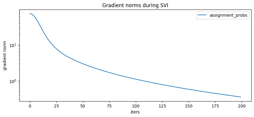
在训练期间,我们将收集损失和梯度范数以监控收敛情况。我们可以使用下面的 hook_optax 辅助函数来完成。
[5]:
# Helper function to collect gradient norms during training
def hook_optax(optimizer):
    gradient_norms = defaultdict(list)

    def append_grad(grad):
        for name, g in grad.items():
            gradient_norms[name].append(float(jnp.linalg.norm(g)))
        return grad

    def update_fn(grads, state, params=None):
        grads = pure_callback(append_grad, grads, grads)
        return optimizer.update(grads, state, params=params)

    return optax.GradientTransformation(optimizer.init, update_fn), gradient_norms


optim, gradient_norms = hook_optax(optax.adam(learning_rate=0.1, b1=0.8, b2=0.99))
global_svi = SVI(model, global_guide, optim, loss=elbo)
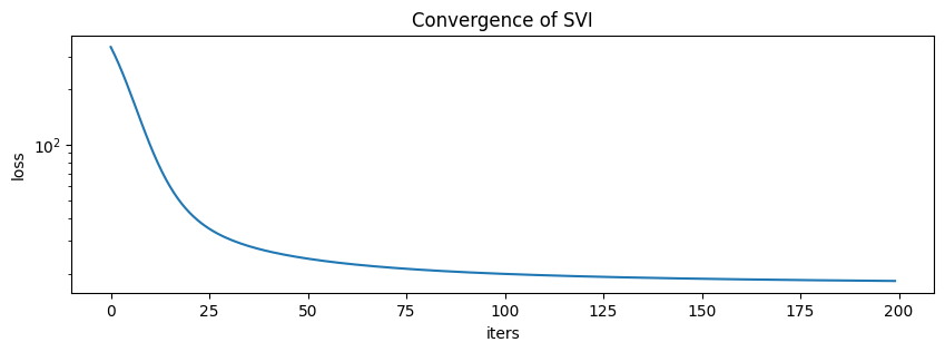
现在训练模型
[6]:
global_svi_result = global_svi.run(
    random.PRNGKey(0), 200 if not smoke_test else 2, data
)
100%|███████████████████████████████████████████████████████████████████████████| 200/200 [00:00<00:00, 287.42it/s, init loss: 25.1498, avg. loss [191-200]: 17.4433]
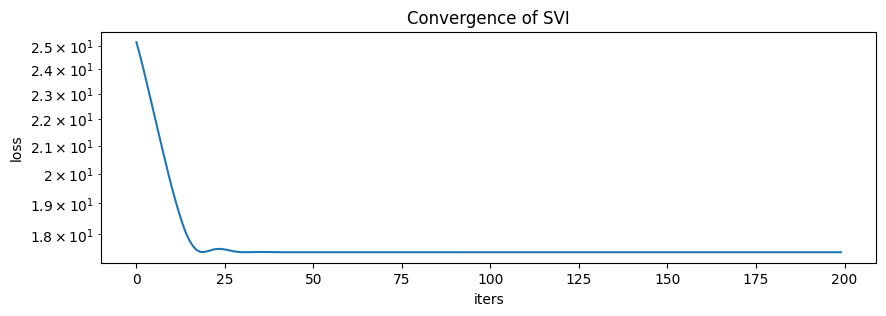
[7]:
plt.figure(figsize=(10, 3), dpi=100).set_facecolor("white")
plt.plot(global_svi_result.losses)
plt.xlabel("iters")
plt.ylabel("loss")
plt.yscale("log")
plt.title("Convergence of SVI")
plt.show()
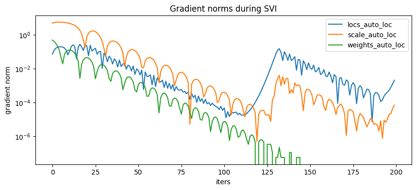
[8]:
plt.figure(figsize=(10, 4), dpi=100).set_facecolor("white")
for name, grad_norms in gradient_norms.items():
    plt.plot(grad_norms, label=name)
plt.xlabel("iters")
plt.ylabel("gradient norm")
plt.yscale("log")
plt.legend(loc="best")
plt.title("Gradient norms during SVI")
plt.show()
这是学到的参数
[9]:
map_estimates = global_svi_result.params
weights = map_estimates["weights_auto_loc"]
locs = map_estimates["locs_auto_loc"]
scale = map_estimates["scale_auto_loc"]
print(f"weights = {weights}")
print(f"locs = {locs}")
print(f"scale = {scale}")
weights = [0.375 0.625]
locs = [ 0.4989534 10.984944 ]
scale = 0.6514341831207275
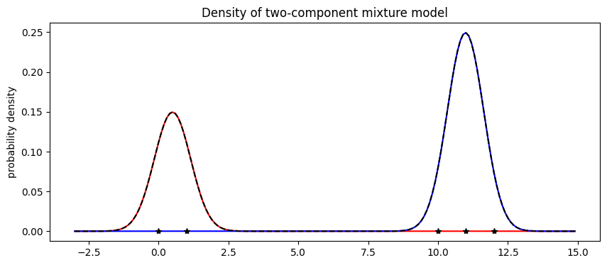
模型学习到的 weights 与预期一致,约 2/5 的数据在第一个分量中,3/5 在第二个分量中。接下来我们可视化混合模型。
[10]:
X = jnp.arange(-3, 15, 0.1)
Y1 = weights[0] * scipy.stats.norm.pdf((X - locs[0]) / scale)
Y2 = weights[1] * scipy.stats.norm.pdf((X - locs[1]) / scale)

plt.figure(figsize=(10, 4), dpi=100).set_facecolor("white")
plt.plot(X, Y1, "r-")
plt.plot(X, Y2, "b-")
plt.plot(X, Y1 + Y2, "k--")
plt.plot(data, jnp.zeros(len(data)), "k*")
plt.title("Density of two-component mixture model")
plt.ylabel("probability density")
plt.show()
最后请注意,混合模型的优化是非凸的,并且经常会陷入局部最优。例如,在本教程中,我们观察到如果 scale 初始化得太大,混合模型就会陷入所有数据都在一个簇中的假设。
模型服务:预测成员关系
既然我们已经训练了一个混合模型,我们可能想将该模型用作分类器。在训练过程中,我们边缘化了模型中的分配变量。虽然这提供了快速收敛,但它阻止了我们从指南中读取簇分配。我们将讨论将模型视为分类器的两种选择:第一种是使用 infer_discrete(快得多),第二种是通过在 SVI 中使用枚举来训练辅助指南(较慢但更通用)。
使用离散推断预测成员关系
预测成员关系的最快方法是使用 infer_discrete 处理器,结合 trace 和 replay。我们先从一个 MAP 分类器开始,将 infer_discrete 的温度参数设为零。要深入了解像 trace、replay 和 infer_discrete 这样的效果处理器,请参阅效果处理器教程。
[11]:
trained_global_guide = handlers.substitute(
    global_guide, global_svi_result.params
)  # substitute trained params
guide_trace = handlers.trace(trained_global_guide).get_trace(data)  # record the globals
trained_model = handlers.replay(model, trace=guide_trace)  # replay the globals


def classifier(data, temperature=0, rng_key=None):
    inferred_model = infer_discrete(
        trained_model, temperature=temperature, first_available_dim=-2, rng_key=rng_key
    )  # set first_available_dim to avoid conflict with data plate
    seeded_inferred_model = handlers.seed(inferred_model, random.PRNGKey(0))
    trace = handlers.trace(seeded_inferred_model).get_trace(data)
    return trace["assignment"]["value"]


print(classifier(data))
[0 0 1 1 1]
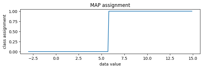
确实,我们可以在新数据上运行这个分类器
[12]:
new_data = jnp.arange(-3, 15, 0.1)
assignment = classifier(new_data)
plt.figure(figsize=(8, 2), dpi=100).set_facecolor("white")
plt.plot(new_data, assignment)
plt.title("MAP assignment")
plt.xlabel("data value")
plt.ylabel("class assignment")
plt.show()
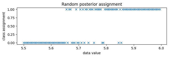
要生成随机后验分配而非 MAP 分配,我们可以设置 temperature=1。
[13]:
print(classifier(data, temperature=1, rng_key=random.PRNGKey(0)))
[0 0 1 1 1]
由于类别分隔得非常开,我们放大到类别边界附近,大约 5.75。
[14]:
new_data = jnp.arange(5.5, 6.0, 0.005)
assignment = classifier(new_data, temperature=1, rng_key=random.PRNGKey(0))
plt.figure(figsize=(8, 2), dpi=100).set_facecolor("white")
plt.plot(new_data, assignment, "x", color="C0")
plt.title("Random posterior assignment")
plt.xlabel("data value")
plt.ylabel("class assignment")
plt.show()
通过在指南中枚举来预测成员关系
预测类别成员关系的第二种方法是在指南中进行枚举。这对于服务分类器模型效果不佳,因为我们需要为每个新的输入数据批次运行随机优化,但它更通用,因为它可以嵌入到更大的变分模型中。
为了从指南中读取簇分配,我们将定义一个新的 full_guide,它同时拟合全局参数(如上所述)和局部参数(以前已被边缘化)。由于我们已经为全局变量学习到了良好的值,我们将通过使用 handlers.block 来阻止 SVI 更新它们。
[15]:
@config_enumerate
def full_guide(data):
    # Global variables.
    with handlers.block(
        hide=["weights_auto_loc", "locs_auto_loc", "scale_auto_loc"]
    ):  # Keep our learned values of global parameters.
        trained_global_guide(data)

    # Local variables.
    with numpyro.plate("data", len(data)):
        assignment_probs = numpyro.param(
            "assignment_probs",
            jnp.ones((len(data), K)) / K,
            constraint=constraints.simplex,
        )
        numpyro.sample("assignment", dist.Categorical(assignment_probs))
[16]:
optim, gradient_norms = hook_optax(optax.adam(learning_rate=0.2, b1=0.8, b2=0.99))
elbo = TraceEnum_ELBO()
full_svi = SVI(model, full_guide, optim, loss=elbo)


full_svi_result = full_svi.run(random.PRNGKey(0), 200 if not smoke_test else 2, data)
100%|██████████████████████████████████████████████████████████████████████████| 200/200 [00:00<00:00, 298.62it/s, init loss: 338.6479, avg. loss [191-200]: 18.2659]
[17]:
plt.figure(figsize=(10, 3), dpi=100).set_facecolor("white")
plt.plot(full_svi_result.losses)
plt.xlabel("iters")
plt.ylabel("loss")
plt.yscale("log")
plt.title("Convergence of SVI")
plt.show()
[18]:
plt.figure(figsize=(10, 4), dpi=100).set_facecolor("white")
for name, grad_norms in gradient_norms.items():
    plt.plot(grad_norms, label=name)
plt.xlabel("iters")
plt.ylabel("gradient norm")
plt.yscale("log")
plt.legend(loc="best")
plt.title("Gradient norms during SVI")
plt.show()
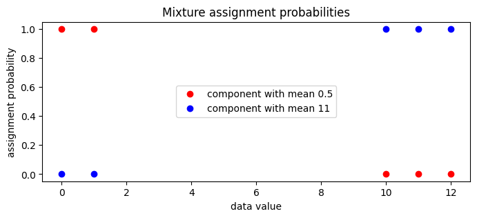
现在我们可以检查指南的局部 assignment_probs 变量。
[19]:
assignment_probs = full_svi_result.params["assignment_probs"]
plt.figure(figsize=(8, 3), dpi=100).set_facecolor("white")
plt.plot(
    data,
    assignment_probs[:, 0],
    "ro",
    label=f"component with mean {locs[0]:0.2g}",
)
plt.plot(
    data,
    assignment_probs[:, 1],
    "bo",
    label=f"component with mean {locs[1]:0.2g}",
)
plt.title("Mixture assignment probabilities")
plt.xlabel("data value")
plt.ylabel("assignment probability")
plt.legend(loc="center")
plt.show()
MCMC
接下来,我们将使用折叠 NUTS 探索分量参数的完整后验,即我们将使用 NUTS 并边缘化所有离散潜在变量。
[20]:
from numpyro.infer import MCMC, NUTS

kernel = NUTS(model)
mcmc = MCMC(kernel, num_warmup=50, num_samples=250)
mcmc.run(random.PRNGKey(2), data)
mcmc.print_summary()
posterior_samples = mcmc.get_samples()
sample: 100%|███████████████████████████████████████████████████████████████████████████| 300/300 [00:02<00:00, 130.21it/s, 7 steps of size 2.44e-01. acc. prob=0.41]
                mean       std    median      5.0%     95.0%     n_eff     r_hat
   locs[0]      2.45      4.30      0.62     -0.97     11.41      8.92      1.14
   locs[1]      8.72      4.19     10.75      0.23     11.78      8.12      1.16
     scale      1.58      1.75      1.02      0.57      3.46     19.19      1.02
weights[0]      0.47      0.20      0.48      0.17      0.76      8.78      1.03
weights[1]      0.53      0.20      0.52      0.24      0.83      8.78      1.03

Number of divergences: 11
[21]:
X, Y = posterior_samples["locs"].T
[22]:
plt.figure(figsize=(8, 8), dpi=100).set_facecolor("white")
h, xs, ys, image = plt.hist2d(X, Y, bins=[20, 20])
plt.contour(
    jnp.log(h + 3).T,
    extent=[xs.min(), xs.max(), ys.min(), ys.max()],
    colors="white",
    alpha=0.8,
)
plt.title("Posterior density as estimated by collapsed NUTS")
plt.xlabel("loc of component 0")
plt.ylabel("loc of component 1")
plt.tight_layout()
plt.show()
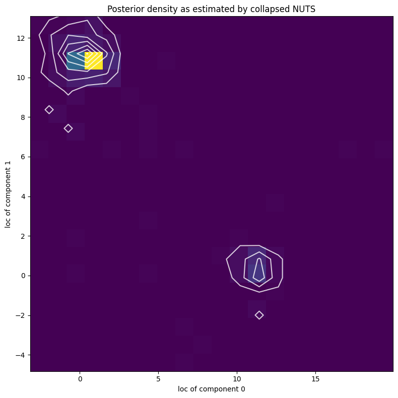
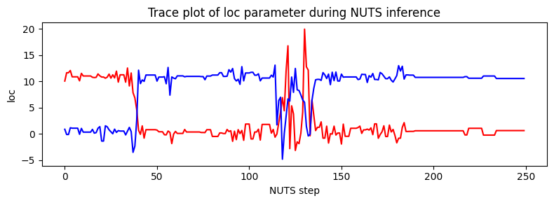
请注意,由于混合分量的不可辨识性,似然曲面有两个同样可能的模态,靠近 (11,0.5) 和 (0.5,11)。NUTS 在两个模态之间切换存在困难。
[23]:
plt.figure(figsize=(8, 3), dpi=100).set_facecolor("white")
plt.plot(X, color="red")
plt.plot(Y, color="blue")
plt.xlabel("NUTS step")
plt.ylabel("loc")
plt.title("Trace plot of loc parameter during NUTS inference")
plt.tight_layout()
plt.show()